(Haskell in Haskell) 4. Simplification

In this post we’ll be writing a simplifier for our subset of Haskell. We’ll be transforming and trimming down our AST to make it more suitable for type-checking, and easier to convert to lower-level representations.

So far, we’ve mainly been working on what’s called the frontend of our compiler. This goes from the source code that the user deals with, and gives us a representation of that code we can work with. Now we’re starting work on the middle part of our compiler, which analyzes and transforms this representation, preparing it for the backend, which will generate the C so that our program can be executed.

We’ll be going over a handful topics:

• What does our simplifier need to do anyways?
• What kind of information do we need for the types defined in our program?
• How do we resolve the type synonyms that the user created?
• What redundant parts of the syntax tree can be rewritten?
• How do we unify multiple function heads into simple case expressions?

By the end of this post, we’ll have seen approaches to these questions and problems, and created a compiler stage putting these ideas into practice.

What our simplifier needs to do

Our main goal for this part is creating a simplifier. But what is this simplifier trying to accomplish in the first place? There’s no single answer, because the simplifier is ultimately a stage that exists to tie a few loose knots and tidy up a few things we’ve left open after the parsing stage.

Right now, after parsing, our representation of the code is very similar to the source code we’ve just extracted it from. What we aim to do in this stage is to transform this source level representation into something that’s much easier to work with for the stages that come after us.

We’ll need to untangle type and value information, which are currently mixed in our representation, in the same way that Haskell lets you define both types and values in the same file. We’ll also be streamlining our representation of values, simplifying the various constructs in our language, and desugaring a lot of the syntax that our parser previously left untouched.

We’ll also be taking this opportunity to do some basic checks on the integrity of our code, reporting different errors as we transform our syntax tree. These errors are natural extensions of the kind of transformations we want to do.

Type Information

As we’ve just gone over, Haskell mixes type information and value information, and one goal of this stage is going to be to untangle the two parts.

Take a snippet of Haskell like this:

type X = Int
 
data MyData = MyData X
 
x :: MyData
x = MyData 3

Here we have 4 items of interest:

1. The type synonym X = Int
2. A data definition creating a new type MyData
3. A type annotation for x
4. A value definition for x

Items 1 and 2 are squarely in the realm of types, and 4 in the realm of values. Item 3 gives us a type for this value.

One inconvenient aspect of our current representation is that all of these kinds of things are scattered throughout our source code, without any clean separation or organization.

The first problem is that the potential type annotation for a value is separate from that value. In fact, values can be declared multiple times, to allow us to provide pattern matching, like:

add 0 0 = 0
add n m = n + m

We’ll want to unify all the definitions of add into one part of our syntax tree, and bring it together with whatever type annotation it might have had.

We also don’t really need to lug around the syntax for all the type information the user is providing us. What we really want to do is to distill all of this information and only keep track of the parts we need for later.

Type Synonyms

Type synonyms don’t actually need to be kept around, if you think about it. When we create a type synonym and use it:

type X = Int
 
add :: X -> X -> X

what we’re really saying is that this program is equivalent to:

add :: Int -> Int -> Int

and the type synonym can be eliminated completely for later stages.

This applies equally even if that synonym is used inside of a data type:

type X = Int
 
data MyData = MyData X

This program can be replaced with:

data MyData = MyData Int

without changing its meaning at all.

So, we can really discard all of the type synonyms, but only after we’ve replaced all of their occurrences with a fully resolved type. We need to be careful here, since type synonyms can reference other synonyms:

type X = Y
type Y = Z
type Z = Int

We can’t simply make a map Synonym -> ResolvedType by looking at each synonym in the file. Instead we’ll need to do a bit more work to figure out what this map looks like. Regardless, we’ll be using a map like this to eliminate all of the synonyms eventually, and we can discard that map before the next stage, since every type will have been fully resolved.

Note:

If you want to provide nicer errors to the user, then you actually do want to keep this map around, so that you can reference the type synonms that a user provided when talking about errors.

For example, if you have:

type X = Int
 
x :: X
x = "foo"

It’d be nice to say something like “couldn’t match type X with String” than “couldn’t match type Int with String”, since it’s closer to the code the user provided.

Constructor Information

The remaining bit of type information we need to keep track of are the new data types defined by the user. When we have some data type like:

data List a = Cons a (List a) | Nil

we’ll then need to keep track of the two constructors:

Nil :: List a
Cons :: a -> List a -> List a

We can’t get rid of these just yet, since we need to use them for type checking in the next stage. After all, we need to recognize bad usages, like:

Cons 3 3

for example.

Redundancy

So, we want to extract out the type information strewn across our program, but what about the values? We’re not going to leave them untouched either.

As mentioned a few times in the last post, our syntax tree after parsing is very close to the syntax of the language, and has quite a few redundant constructs. These constructs exist because there is syntax for them, and not because they represent truly distinct programs.

Another major goal in our simplifier is going to be trimming the fat on our syntax tree, and simplifying away all of this redundancy.

Let vs Where

The first bit of redundant syntax are let expressions and where expressions. Syntactically, these are different, but they really express the same thing. We can represent a where expression like:

x + y
  where
    x = 2
    y = 3

using let instead:

let x = 2
    y = 3
in x + y

By doing this throughout our syntax tree, we get rid of one superfluous constructor in our tree, which simplifies our work throughout the remaining stages of our compiler.

Lambdas

Syntactically, we allow lambdas with multiple parameters at once:

\x y -> x + y

Our syntax tree represents this verbatim, as:

LambdaExpr ["x", "y"] (BinExpr Add (NameExpr "x") (NameExpr "y"))

It’s common knowledge that this snippet of Haskell is equivalent to:

\x -> \y -> x + y

And we could have parsed our original expression as:

LambdaExpr ["x"] (LambdaExpr ["y"] ...)

matching the second version. We’ve chosen to stick closer to the syntax in our parser, but our simplifier will get rid of these variants, having lambda expressions only take a single parameter, using multiple nested lambdas for multiple parameters.

Applications

In the same way that lambda expressions with multiple parameters can be represented as a sequence of curried lambdas, function application with multiple parameters is also sugar for curried application. For example:

add 1 2

is syntax sugar for:

(add 1) 2

Our simplifier is going to take care of this as well. In our parser, applications take multiple parameters, but now we’re going to always represent things as:

Apply f e

where f is our function, and e our expression. For multiple parameters, we just use currying:

Apply (Apply add 1) 2

Note:

I’m using a bit of pseudo-syntax here, but we’ll precisely define the structure of our new AST soon enough.

Builtins

In real Haskell, you have custom operators, and this entails making operators actually functions. So something like:

1 + 2 + 3

is actually lingo for:

(+) (((+) 1) 2) 3

(with the specific ordering dependent on the fixity of the operator, of course)

We’ve opted to instead hardcode the various operators we’re going to be using. We’d represent this same expression as:

BinExpr Add (BinExpr Add 1 2) 3

having simplified the tree a bit.

Instead of using function application, we have a specific syntactical form for operators. What we want to do in our simplifier is to shift this slightly, to reuse function application:

Apply (Builtin Add) (Apply (Builtin Add) 1 2) 3

Instead of having a special form for using operators, we now use function application, and our operators become expression in their own right. We also need to apply currying here, as mentioned in the previous step.

Doing things this way simplifies the next stages quite a bit. We don’t have this extra kind of expression to deal with. For example, in the typechecker, we just treat Builtin Add as an expression of type Int -> Int -> Int, as if it were a named function that happened to be defined.

This is in some sense arriving at the same point Haskell does, where after parsing, operators become the application of certain functions. The difference is that we’ve hardcoded certain functions as existing, and these functions are now builtin to the compiler.

Multiple Function Heads

So, there are quite a few things we can simplify about expressions, but we also have a lot on our plate when it comes to definitions. As mentioned before, the definition for a given value can be spread out over multiple places:

add :: Int -> Int -> Int
add 0 0 = 0
add n m = n + m

In this example, the definition of add is separated across 3 different elements. We have one type annotation:

add :: Int -> Int -> Int

one definition using pattern matching:

add 0 0 = 0

and a second definition using pattern matching, but with simple name patterns:

add n m = n + m

Our first order of duty is going to be to somehow unify these three different items into a single definition. We want each value definition in our program to correspond to a single item in our simplified tree.

To accomplish this we need to first gather all of the definitions of a value, along with its type annotation. We can do a few integrity checks here, like making sure that each definition has the same number of arguments, that multiple type annotations exist, etc. Then we simplify this collection into a single definition, which requires a couple of things.

Creating Functions

There are multiple ways of defining a function like add above:

add n m = n + m
 
add n = \n -> n + m
 
add = \n -> \m -> n + m

All of these are equivalent. The first definition is really syntax sugar for the last definition. What we want to do is transform functions declaring parameters like this to bindings of a name to a simple lambda instead.

Multi Cases

The last change was pretty simple, but this one is a bit more complicated. The idea is that in the same way that we transform simple names on the left side of = into lambdas on the right side, we also need to transform patterns like this:

inc 0 = 1
inc x = x + 1

into lambdas and case expressions:

inc = \$0 -> case $0 of
  0 -> 1
  x -> x = 1

This is straightforward so far, and easy to see. The problem comes with how functions can match on multiple values. This isn’t possible with case expressions.

Note:

One solution to this problem is to simply create a case construction allowing us to match on multiple values at once, punting the problem this poses until after the type-checker.

I opted against doing this, because by tackling this complexity now it makes the type-checker simpler as well.

For example, take our ongoing example:

add 0 0 = 0
add n m = n + m

If we try and desugar this as we did previously, we have a problem:

add = \$0 -> \$1 -> case ? of

We can’t simply move each of the patterns we had previously, since we have no way matching against both values at the same time. What we need to do is figure out a way of nesting our case expressions. In this case, there’s a pretty simple solution:

add = \$0 -> \$1 ->
  case $0 of
    0 -> case $1 of
      0 -> 0
      m -> $0 + m
    n -> n + $1

It’s not too hard to translate things like this manually. The difficult comes from doing this automatically. We want to write an algorithm to perform conversions like this.

Simplifying Cases

Another detail we’ll be tackling at the same time is removing nested cases completely. Right now, we can do things like this:

data List a = Cons a (List a) | Nil
 
drop3 :: List a -> List a
drop3 = \xs -> case xs of
  Cons _ (Cons _ (Cons _ rest)) -> rest
  _ -> Nil

This function drops off 3 elements from the front of a list. To do this, we need to use multiple nested patterns, in order to match against the tail of different lists.

In fact, we allow arbitrary patterns to be used inside of a constructor.

We’re going to be simplifying case expressions like this, to only use simple patterns inside of constructors. One way of simplifying this would be:

drop3 = \xs -> case xs of
  Nil -> Nil
  Cons _ $0 -> case $0 of
    Nil -> Nil
    Cons _ $1 -> case $1 of
      Nil -> Nil
      Cons _ rest -> rest

Once again, we can do this by hand without all that much effort, but the trickiness comes from being able to do this automatically.

In fact, we’ll be felling two birds with one stone here. We’ll write an algorithm that converts multiple nested pattern matching, into single pattern matching without any nesting. This way, we can tackle the problems of patterns in functions, and simplifying normal case expressions with the same tool.

Note:

We do this not out of necessity, but because we need to do this eventually, and getting this out of the way now is convenient, since we already need to apply a simplification algorithm to our cases, to remove multiple pattern matching in functions.

Doing this now allows us to simplify the type-checker. Otherwise, we’d have to do all of this afterwards.

Creating a Stub Simplifier

As usual for this series, we’re going to start by creating a dummy module for our Simplifier, and integrating it with the rest of the compiler, before coming back and slowly filling out its various components.

Let’s go ahead and add a Simplifier module to our .cabal file:

  exposed-modules:     Ourlude
                     , Lexer
                     , Parser
                     , Simplifier
                     , Types

Next, let’s create our actual module in src/Simplifier.hs

{-# LANGUAGE FlexibleContexts #-}
{-# LANGUAGE GeneralizedNewtypeDeriving #-}
{-# LANGUAGE LambdaCase #-}
{-# LANGUAGE TupleSections #-}
 
module Simplifier
  ( AST (..),
    SimplifierError (..),
    simplifier,
  )
where
 
import Ourlude
import qualified Parser as P

We have the standard import for our Prelude, of course, and a qualified import to be able to easily access everything in our parser stage. We’ll be expanding this with other imports as necessary.

Except for FlexibleContexts, we’ve seen all of these extensions before.

We’ll be using FlexibleContexts to work with some typeclasses that take multiple types, namely MonadError. This extension allows us to write constraints like:

doSomething :: MonadError Concrete generic => ...

In this example, we use a concrete type inside of a constraint, which is enabled by FlexibleContexts.

AST is going to be the simplified syntax tree eventually, but we can just create a stub value for now:

data AST t = AST deriving (Show)

The parameter t will eventually be used to hold the kind of type stored in the AST. This isn’t used right now, but will be soon enough.

We’ll be needing a type for the errors emitted by this stage, so let’s go ahead and create the SimplifierError type as well:

data SimplifierError = NotImplementedYet deriving (Eq, Show)

This is just a stub type for now, indicating that we haven’t implemented this stage yet. We’ll be coming back to this type and actually adding useful errors later.

The last thing we’ll be adding for now is our stage function:

simplifier :: P.AST -> Either SimplifierError (AST ())
simplifier _ = Left NotImplementedYet

For now, we just report an error, since we haven’t implemented anything yet. Note how we use AST () here. This is because after the simplification stage, we haven’t done any type inference, so we use the type () for the types in our AST. The type-checker will be filling these slots with something useful, but that’s for the next part.

Adding a new Stage

With this stub stage defined, we can go ahead and integrate it with the rest of our CLI.

Inside of Main.hs, let’s import our newly created module:

import qualified Simplifier

Let’s now create a stage object for the Simplifier:

simplifierStage :: Stage Parser.AST (Simplifier.AST ())
simplifierStage = makeStage "Simplifier" Simplifier.simplifier

Finally, let’s modify readStage to include this stage as an additional option:

readStage :: String -> Maybe String -> Maybe (String -> IO ())
readStage "lex" _ =
  lexerStage |> printStage |> Just
readStage "parse" _ =
  lexerStage >-> parserStage |> printStage |> Just
readStage "simplify" _ =
  lexerStage >-> parserStage >-> simplifierStage |> printStage |> Just

We can now run this new command in the terminal:

$ cabal run haskell-in-haskell -- simplify foo.hs
Up to date
Simplifier Error:
NotImplementedYet

As expected, we immediately report an error in our simplifier stage. To fix this, we need to actually implement our simplifier stage!

Schemes

Our next goal is to define the kinds of type information that our simplifier needs to gather from our parsed program. Before we can do that, however, we need to expand our vocabulary around types a bit more.

At the moment, we have a module for type related data, defined in src/Types.hs. All of the things we’ve defined in there so far were necessary to talk about types syntactically. If we see:

f :: Int -> Int

Then we need a way to talk about the type Int -> Int, in our own compiler. Concretely, we represent this as IntT :-> IntT, in our Type data structure.

We also included variables, allowing us to talk about polymorphic function signatures:

id :: a -> a

We’d represent this type signature as:

TVar "a" :-> TVar "a"

The polymorphic variable a is implicit in this type signature. We never declare the variable at all, but (our subset of) Haskell knows that we mean a polymorphic signature, because the a is lowercase. The signature A -> A would be quite different, referencing a concrete type A, which would have to be defined somewhere else.

In actual Haskell, you could instead write id’s signature with an explicit polymorphic variable:

id :: forall a. a -> a

We don’t allow this syntactically, but after the simplifier stage, we’d like to resolve the implicit polymorphism we have now, and move towards explicitly qualified polymorphism.

We call these kinds of things schemes (No relation to algebraic geometry).

We want to be able to represent different signatures, like:

forall a. a -> a
forall a b. a -> b -> b

etc.

Defining Them

So, in src/Types.hs, let’s go ahead and create a definition for a Scheme:

data Scheme = Scheme [TypeVar] Type deriving (Eq, Show)

Note that TypeVar and Type have already been defined by us previously. We’re just saying that a scheme is nothing but some type, referencing a list of explicitly defined variables.

For example, the signature forall a. a -> a would be represented as:

Scheme ["a"] (TVar "a" :-> TVar "a")

Note:

Strictly speaking, we could’ve represented a scheme as a type, quantified with a set of type variables, instead of a list, as we’ve done here.

Having a list is slightly more convenient, and more conventional. In practice, this list is going to be unique, having been created from a set.

Using Them

We can go ahead and define a few useful operations on Schemes, that we’ll be needing later on. The main operation we’d like to have is one going from an implicit signature like:

a -> b -> b

into an explicit Scheme:

forall a b. a -> b -> b

All we need to do is make a list of all the different variables appearing in that type signature. We call the variables that appear unbound in a signature like this “free”. Not only can we look at the free variables in some type, but this concept also makes sense for schemes. For example, a scheme like:

forall a. a -> b -> b

Only quantifies over a. The variable b is “free” inside of this scheme. At the top level, this kind of thing doesn’t occurr, but we will actually be making use of this for inferring types inside of definitions, where intermediate definitions can make use of type variables defined in the outer scope. We’ll be seeing all of that in the next part, when we focus on type-checking. For now, let’s just realize that the different data structures might contain free type variables in one way or another.

Because we have a similar operation across different types, let’s create a class for different things containing free type variables:

import qualified Data.Set as Set
-- ...
 
class FreeTypeVars a where
  ftv :: a -> Set.Set TypeName

(We need to use the Set data structure, and so need an extra import now)

This class allows us to extract a set containing the names of the free type variables occurring in an object.

Let’s implement this for types:

instance FreeTypeVars Type where
  ftv IntT = Set.empty
  ftv StringT = Set.empty
  ftv BoolT = Set.empty
  ftv (TVar a) = Set.singleton a
  ftv (t1 :-> t2) = ftv t1 <> ftv t2
  ftv (CustomType _ ts) = foldMap ftv ts

For types, since they don’t introduce any type variables themselves, any type variable ocurring inside of a type is free by definition. This function just has to find the set of type variables contained inside of this type.

For primitives, they obviously contain no type variables. A type variable gives us a single set, containing just that variable, and other composite types have us take the unions of all the variables in each part. This way, ftv (TVar "a" :-> TVar "b") correctly detects both type variables contained inside this function signature.

Out of convenience, we can also give an instance for TypeName:

instance FreeTypeVars TypeName where
  ftv = Set.singleton

Seeing a name "a" as lingo for TVar "a", the free variables occurring in this “type” are just this one variable.

Things get a bit more interesting for schemes:

instance FreeTypeVars Scheme where
  ftv (Scheme vars t) = Set.difference (ftv t) (Set.fromList vars)

Since a scheme like forall a. a -> b -> b introduces a type variable a, we need to remove it from all of the variables that ocurr in the type a -> b -> b, leaving us with just the set {b}.

Finally, it’d be nice to take a set of objects containing type variables, and get the union of all the variables containing in this big bag.

To do so, let’s first add a languag extension at the top of this file:

{-# LANGUAGE FlexibleInstances #-}

which is required to even declare the following instance:

instance FreeTypeVars a => FreeTypeVars (Set.Set a) where
  ftv = foldMap ftv

Once again, we use the fact that <> for sets takes the union, allowing us to take all of the type variables strewn throughout a collection of objects.

With all of this in place, we can go ahead and make the original operation we wanted to make in this section: making all the variables in some type explicitly quantified:

closeType :: Type -> Scheme
closeType t = Scheme (ftv t |> Set.toList) t

This takes some type signature, like a -> a, potentially containing implicit polymorphism, and then explicitly quantifies over all the type variables occurring in that signature. An obvious application of this is transforming top level signatures like:

id :: a -> a

into explicit signatures like:

id :: forall a. a -> a

With all of this scheme stuff in place, we can move on to defining the type information produced by our simplifier.

Defining Type Information

As we went over earlier, our simplifier will need to gather information about the types in our program. Before we write code to do the actual gathering, let’s first define what kind of information we want to gather in the first place, and write some utilities to make use of this information.

Now that we’re actually doing interesting things in our simplifier module, let’s go ahead and add all the imports we’ll be needing

import Control.Monad (forM_, replicateM, unless, when)
import Control.Monad.Except (Except, MonadError (..), liftEither, runExcept)
import Control.Monad.Reader (MonadReader (..), ReaderT (..), ask, asks, local)
import Control.Monad.State (MonadState, StateT (..), execStateT, get, gets, modify', put)
import Data.Foldable (asum)
import Data.Function (on)
import Data.List (elemIndex, foldl', groupBy, transpose)
import qualified Data.Map as Map
import Data.Maybe (catMaybes)
import qualified Data.Set as Set
import Ourlude
import Parser (ConstructorDefinition (..), ConstructorName, Literal (..), Name, ValName)
import qualified Parser as P
import Types (FreeTypeVars (..), Scheme (..), Type (..), TypeName, TypeVar, closeType)

We have quite a few imports related to different Monad Transformers, and related utilities. We won’t be using these immediately, but our transformations will be making good use of these transformers later on.

We need the Map and Set data structures as well, along with a few related utilities from various modules.

We also import a handful of types directly from our parser, and then import the rest of the parser module in a qualified way.

Finally, we import most of everything from src/Types.hs, including the newly defined scheme type.

Constructor Information

If a user defines a custom type, like:

data MyType = MyPair Int String | MySingle

We have two constructors, MyPair, and MySingle, and it’s nice to have some information about them available for the later stages. For example, our type checker needs to know that each constructor has a given type:

MyPair :: Int -> String -> MyType
MySingle :: MyType

We would also like to assign a “tag” to each constructor of a type. For example, if we have a simple enum, like:

data Color = Red | Blue | Green

then to distinguish the different variants, we might represent this type as just an integer, with a different tag for each variant:

Red = 0
Blue = 1
Green = 2

The way we assign a tag to each variant doesn’t matter too much, as long as each variant gets a different tag.

Let’s define a ConstructorInfo type, holding the information we’d like to know about any given constructor:

data ConstructorInfo = ConstructorInfo
  { constructorArity :: Int,
    constructorType :: Scheme,
    constructorNumber :: Int
  }
  deriving (Eq, Show)

We have a number assigned to each constructor. This number is different for each constructor, and can serve the purpose of the “tag” we talked about earlier.

The constructorType field gives us the type of the constructor, as a function. Note that this is polymorphic, and uses a scheme. This lets us do polymorphic constructors, like:

data Pair a b = MkPair a b

The MkPair constructor would have as scheme:

forall a b. a -> b -> Pair a b

Finally, the constructorArity field encodes the number of arguments that a constructor takes. We could derive this from the type signature of the constructor, by looking at the number of arguments the function takes, but it’s convenient to be able to access this information directly, having computed it in advance.

We’d like to gather this information for all of the constructors in the program, and we need to be able to lookup this information for any constructor on demand. So, let’s define the following type synonym:

type ConstructorMap = Map.Map ConstructorName ConstructorInfo

This will map each constructor, to the corresponding information we have about that constructor, using its name.

Resolving Constructors

We’ll be needing this constructor information not just when type checking, but later on in the compiler as well. Because of this, we can make a few generic utilities for contexts which have access to this constructor information:

class Monad m => HasConstructorMap m where
  constructorMap :: m ConstructorMap

The idea behind this class is that in later stages, where we have some kind of Monadic context used to perform some transformation, we might have this constructor information embedded somewhere in this context, and this class lets us abstract over that fact.

A convenient utility we can make using this class is a function letting us check if a given name is a constructor:

isConstructor :: HasConstructorMap m => Name -> m Bool
isConstructor name =
  Map.member name <$> constructorMap

This will be useful in the later STG stage, where we need to distinguish function application from constructor application.

We’ll also be using this information inside of our simplifier. In this case, what should we do if a constructor that doesn’t exist is referenced? Well, we should catch this error in our simplifier! Let’s add a variant to our SimplifierError type:

data SimplifierError
  = UnknownConstructor ConstructorName
  deriving (Eq, Show)

This error should be raised whenever we encounter a constructor that doesn’t exist, as the name suggests.

Outside of the simplifier, we know that the constructors present in the program actually exist, so we can make a utility that looks up a constructor, crashing if this constructor doesn’t exist:

lookupConstructorOrFail ::
  HasConstructorMap m => ConstructorName -> m ConstructorInfo
lookupConstructorOrFail name =
  Map.findWithDefault err name <$> constructorMap
  where
    err = UnknownConstructor name |> show |> error

If this fails after the simplifier stage, then that indicates an error on our part as a compiler writer, since our simplifier stage is responsible for making sure that the constructors used in our program actually exist.

Synonym Information

Now, the types contained in each constructor are going to be resolved, in the sense that all of the type synonyms that might have appeared in the constructor’s signature reference the most basic type.

So, for example:

data MyType = MkMyType X
 
type X = Int

The constructor MkMyType would have signature:

Int -> MyType

and not:

X -> MyType

In fact, all of the types that come out of the simplifier stage will be fully resolved in this fashion.

To accomplish this, we do need to have an internal map from type names like X to the actual type it references. So, let’s define the following synonym:

type ResolutionMap = Map.Map TypeName ResolvingInformation

For each type name, like X, or MyType, we have some information about what kind of type that is. Note that primitive types like Int or Bool are already parsed as syntactically different, as IntT or BoolT, instead of CustomType "Int" [] and CustomType "Bool" [].

But, what kind of information do we have about each type name?

There are two situations we can have. Either a type is a synonym, like type X = Int, or it’s a full type in its own right, like MyType. A name might also reference a polymorphic type, like:

data Pair a b = MkPair a b

In this case, when we see the name Pair, we’d like to record that this is in fact a custom type, and has 2 type parameters.

This gives us the following definition:

data ResolvingInformation
  = Synonym Type
  | Custom Int
  deriving (Eq, Show)

Synonym represents the case where some name represents a synonym for some other type. Note that this is fully resolved, so if we had something like:

type X = Y
type Y = Int

Then both X and Y would resolve to Synonym IntT.

For custom types, we record the number of type arguments that this type takes. This allow us to tell that Pair Int Int Int is malformed, because Pair only takes 2 arguments, as a custom type.

Resolving Types

Internally, we’d like to use this information, and be able to turn types referencing synonyms into fully resolved types, fullfilling our promise of only exporting fully resolved synonyms from this module.

Before we can do that, let’s first add a few more errors to our error type:

data SimplifierError
  = UnknownType TypeName
  | MismatchedTypeArgs TypeName Int Int
  | ...
  deriving (Eq, Show)

UnknownType signals the fact that we’ve encountered some type that doesn’t exist.

MismatchedTypeArgs is raised when we encounter a type name, with a certain expected number of arguments, that doesn’t match the actual number provided.

With these errors in place, we can write a function to resolve any type, replacing synonyms with actual types, provided we have a ResolutionMap:

resolve :: ResolutionMap -> Type -> Either SimplifierError Type
resolve mp = go
  where
    go :: Type -> Either SimplifierError Type
    go = \case
      CustomType name ts -> do
        ts' <- mapM go ts
        let arity = length ts'
        case Map.lookup name mp of
          Nothing -> Left (UnknownType name)
          Just (Synonym _) | arity /= 0 ->
            Left (MismatchedTypeArgs name 0 arity)
          Just (Synonym t) -> return t
          Just (Custom expected) | arity /= expected ->
            Left (MismatchedTypeArgs name expected arity)
          Just (Custom _) -> return (CustomType name ts')
      t1 :-> t2 -> (:->) <$> go t1 <*> go t2
      terminal -> return terminal

(Remember that type synonyms like X will be represented as CustomType "X" [])

Now, we only have work to do if we have a recursive type like :->, or if we have a custom type of some kind. If we have a compound type, we first resolve each of its sub-components.

Then, we lookup the name referenced in the custom type.

If we have no information about the type, then we throw an error.

If it’s a synonym, then we make sure that no extra arguments have been passed. THis is because we don’t allow things like:

data MyPair a b = MkPair a b
 
type P = MyPair

If this is a custom type, we make sure that the number of arguments matches the number we expect to say.

Gathering Synonym Information in Theory

This ResolutionMap would solve all of our problems in terms of type synonyms, but how do we go about actually creating this map in the first place?

Let’s say we have multiple type synonyms in our program:

type X = Int
type Y = String
type Z = Bool

We want to make a map from each type synonym’s name to the actual type that it corresponds to. A first attempt would be to take these definitions, and create a simple direct mapping:

X -> Int
Y -> String
Z -> Bool

This happens to work in this case, but this is because our type synonyms are already fully resolved. It might be the case that our synonyms reference other synonyms:

type X = Int
type Y = X
type Z = Y

If we make a map with these direct mappings once again, we get the wrong result:

X -> Int
Y -> X
Z -> Y

We want to make sure that the mappings we have are fully resolved, so we can’t simply leave X and Y on the right side there.

In this case, the type synonyms are already presented in a convenient order. If we go over the program from top to bottom, we can use the map we’ve built up so far in order to keep building it.

At first, we have:

X -> Int

Then, we see type Y = X. If we resolve the type X, we get Int, since that’s already in the map, giving us:

X -> Int
Y -> Int

Finally, we can do the same with type Z = Y, having resolved Y, giving us:

X -> Int
Y -> Int
Z -> Int

This is the fully resolved map that we needed to make in the first place, so this approach seems promising.

Another difficulty is that the order may not be so convenient. In fact, it’s possible in Haskell to reference type synonyms defined later on in the file:

type X = Int
type Z = Y
type Y = X

Here no simple top to bottom ordering, or bottom to top ordering suffices to resolve things. Instead, we need to make use of the dependencies between different synonyms to make a resolution map.

Type Synonyms as a Graph

If we go back to our initial example:

type X = Int
type Y = X
type Z = Y

We can see this setup as a kind of graph, where each type synonym is connected to the types that it depends on:

This also works if we have a more complicated ordering. This setup:

type X = Int
type Z = Y
type Y = X

Would be represented as:

In both of these graphs, we had a simple linear setup, and it was clear how to order things to make our map easily. We might have a more complex dependency setup, however. Consider the following:

type Z = X
 
type X = Int
 
data D = D Z Y
 
type Y = X

This would lead to the following graph:

At a first glance, it’s not exactly clear what the best order to resolve things in would be.

Topological Sort

Thankfully, other people have actually spent time thinking about this problem, and there’s an elegant solution to the problem. What we’ve been drawing each time is a dependency graph. Each type is connected, via arrows, to all the other types that it depends on, in terms of definitions. What we’d like to find is a linear ordering of the types that respects this chain of dependencies.

If we look at the previous graph, then this ordering:

X <- Z <- Y <- D

would respect the dependencies between each type. After finding this order, we could build up our map of type synonyms in an incremental way, and never run into a type that we haven’t seen before.

Topological sorting is an algorithm that solves our problem exactly. Given some dependency graph, it finds a linear ordering of the vertices that satisfies these dependencies. If the graph has a cycle, this can’t work:

Thankfully, we can also amend the algorithm to detect these cycles, and throw an appropriate error. When we see something like:

type X = Y
type Y = X

We need to throw an error, because there’s no reasonable way to interpret what types X and Y should be.

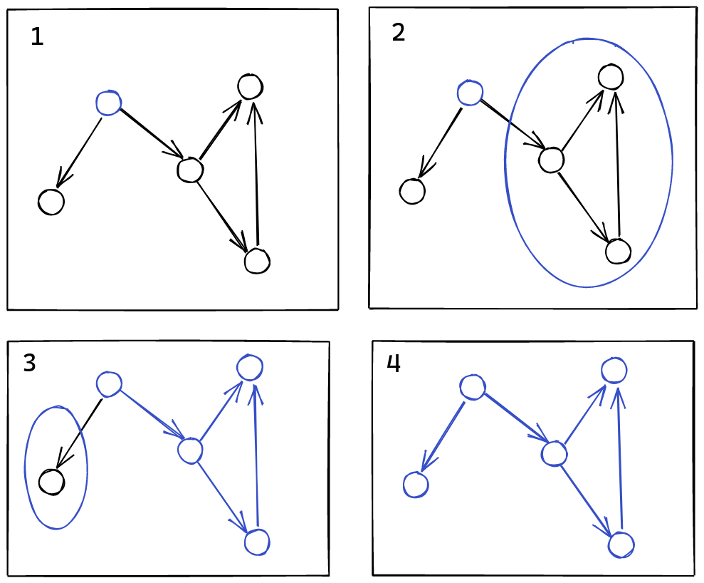
Depth First Search

The key driver of topological sort is something called Depth First Search. This is a way of traversing the nodes in a graph, in a recursive fashion.

Let’s say we have some kind of graph:

We want to visit all of the vertices in a graph, going along the structure of the graph itself. The idea behind depth first search is that we have a recursive function, where to search from a vertex, we mark that vertex as seen, and then recursively search from the vertices directly connected.

More concretely, here’s an illustration of this high level procedure:

We first mark our vertex as seen, that way we won’t visit it again. Then, for each outgoing edge, we follow it, and then repeat the entire search procedure starting from there.

In this case, we end up searching the entire graph, but if we haven’t, we can repeat this procedure, picking a random vertex that we haven’t seen yet.

A complete example of this search procedure would look like this. Every time we see a new vertex, it gets marked in blue, and everytime we traverse an edge, it also gets marked down.

Note that in some cases, we’ve already seen a vertex, so we don’t bother going down some edge again. This is crucial to avoid wasting work, and allowing us to stop the search from going on forever.

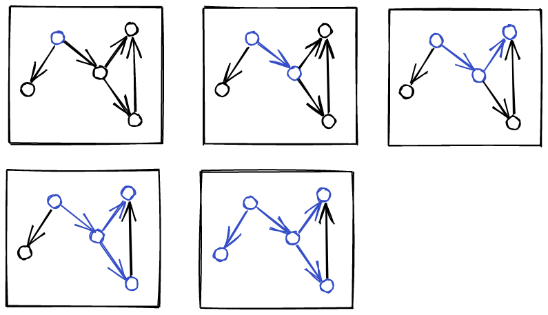
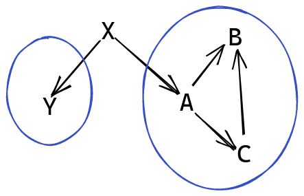
Ordering Vertices

We have a convenient procedure, or at least the idea of a procedure, for traversing the dependency graph, but how can we use this to generate an ordering of these vertices?

The key idea is that all of the dependencies need to come before that vertex.

In this example, we’d make sure to output {A, B, C} in a good order, as well as Y, before finally outputting X. One way to implement this rule, is that after recursing on each outgoing edge, we append the vertex to the list.

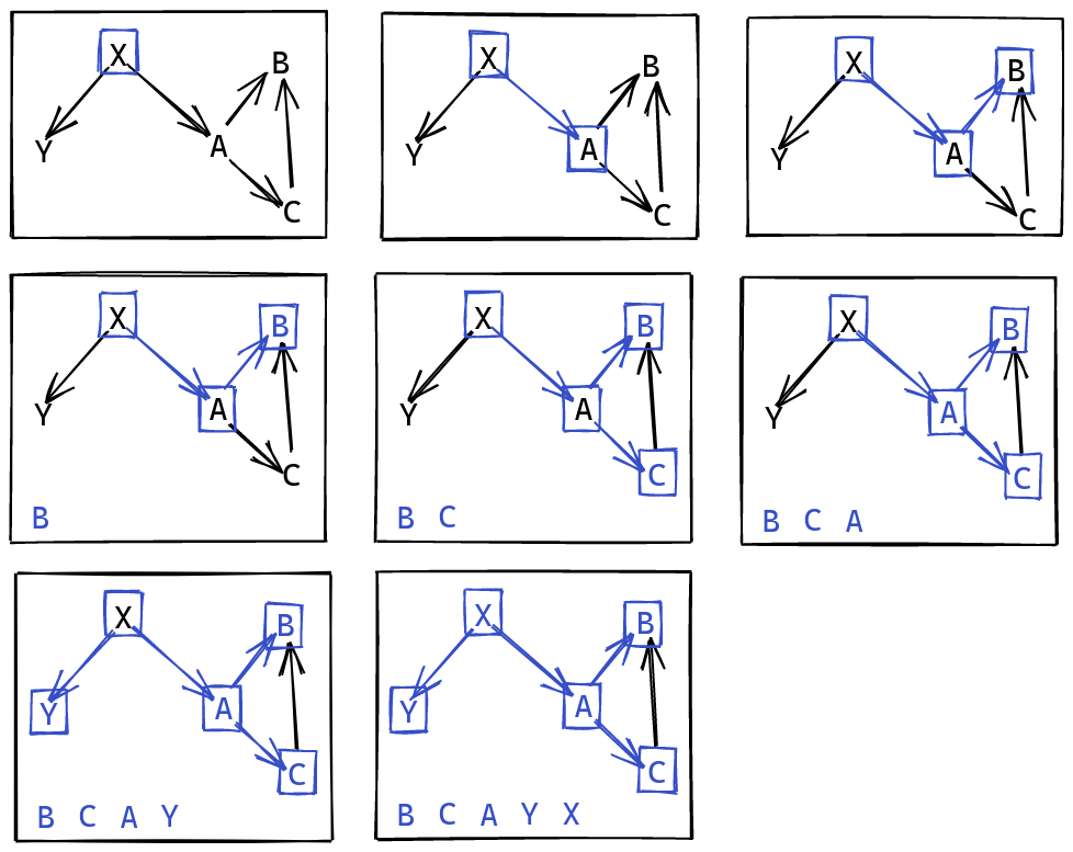
Essentially, this gives us the following procedure:

dfs(vertex):
  seen.insert(vertex)
  for v in neighbors(vertex):
    if not seen.contains(v):
      dfs(v)
  emit(vertex)

We can illustrate this ordering on the graph. We circle a vertex when visited, and mark it when emitted:

The final ordering reflects the dependencies in the graph correctly, because we only emit a vertex after all of is dependents, direct, or indirect, have been emitted as well.

This yields a linear ordering respecting the dependencies.

Note how Y and A B C are independent, and the exact order depends on how we traverse the edges. This is fine, since there are no dependencies between these vertices, if there were, since DFS always recursively traverses as much as possible, we would detect that as well.

Detecting Cycles

This algorithm works great, except when there’s cycles. We can make a slight amendment to this in order to detect cycles. The idea is to simply keep track of a list of ancestors, vertices preceding the current vertex. Then, when visiting a new vertex, we check that it isn’t in this list, otherwise we’d have a cycle:

When visiting a vertex, we mark it as part of the ancestor set, until we’ve finished recursing through all of its outgoing edges.

Well, with that done, we’ve sketched out the algorithm we’ll be using to resolve all of the type synonyms in our program! If this isn’t all that clear, don’t worry too much, since now we get to actually write the code that implements all of this with all the necessary detail.

Gathering Synonyms in practice

In this next section, we’ll be implementing the algorithm we’ve just described. Our end goal is to take the top level definitions produced by our parser, and end up with a ResolutionMap, mapping each type name to either a fully resolved synonym or a known custom type, defined by the user.

The process looks something like this:

1. First, gather all of the type synonyms
2. Sort them, according to the dependency graph
3. Construct the resolutions synonym by synonym, using the partially constructed map

Let’s go ahead and get the sorting out of the way, as that’s somewhat fresh in our mind, and abstracted from the other two steps.

New Errors

First things first, let’s add an extra error variant to SimplifierError:

data SimplifierError
  = CyclicalTypeSynonym TypeName [TypeName]
  | ...
  deriving (Eq, Show)

This error will get thrown if we find a cycle while traversing the graph of type synonyms. We have the type we detected the error at, and a list of ancestors preceding that synonym, making up the cycle.

Sorting Context

Our depth first search algorithm will need to keep track of different pieces of state, as we traverse the graph. We need to keep a set of vertices that we’ve seen so far, crucial to our algorithm. We’ll also be emitting vertices as we do our traversal, so we can keep a list as our “output buffer”.

This gives us the following state for our sorter:

data SorterState = SorterState
  { unseen :: Set.Set TypeName,
    output :: [TypeName]
  }

unseen keeps track of a set of vertices that we have not seen yet. This is more convenient, since it serves both the purpose of the seen set, as well as letting us pick the next vertex to visit, if we run out of neighbors.

The output list lets us emit vertices as we do our traversal, by putting them to the front of the list. We’ll need to reverse the list after we’re finished, of course. Doing it this way is much more efficient than constantly appending to the end of the list.

Inside of our DFS algorithm, we’ll need to be able to modify this state, so we want a monadic context for the sorting algorithm:

type SorterM a =
  ReaderT (Set.Set TypeName)
  (StateT SorterState
  (Except SimplifierError) a)

We have a stateful component for the SorterState type we’ve just defined, allowing us to modify the state as we traverse the graph. We’ll be needing to raise errors, namely if we detect a cycle, so we have a layer for errors with Except as well. We also keep a set of ancestors around, in order to detect cycles.

We could put this information inside of the SorterState, adding and removing ancestors as we start traversing different subgraphs. Using a Reader here lets us temporarily replace the environment before traversing a subgraph, with this change automatically being undone after that recursive call ends. This is more convenient, and a trick we’ll be employing in other stages of the compiler as well.

As usual with monadic contexts, we have a function to run this computation:

runSorter :: SorterM a -> SorterState -> Either SimplifierError a
runSorter m st =
  runReaderT m Set.empty |> (`runStateT` st) |> runExcept |> fmap fst

To run this computation, we just need an initial state to pass in, and we get a value or an error out. This works by passing in an empty set of ancestors, which is the right starting state for our search.

Type Dependencies

We’ve been talking a lot about the “graph” of dependencies. But we don’t actually have a concrete graph lying around. Instead, we look up the dependencies of a type on demand, giving us an implicit graph.

Calculating the dependencies of a type is pretty straightforward:

typeDependencies :: Type -> Set.Set TypeName
typeDependencies = \case
  t1 :-> t2 ->
    typeDependencies t1 <> typeDependencies t2
  CustomType name exprs ->
    Set.singleton name <> foldMap typeDependencies exprs
  _ -> mempty

We have a dependency if we refer to some name anywhere in the type, so we recurse and join together all of the different names referenced in this type.

For example, if we have:

X -> Y

Then X and Y are dependencies of this type.

This also works in nested situations:

List X -> String

Here, List and X are dependencies of this function type.

Core Algorithm

With all of these little pieces on place, we can finally start working on the actual sorting algorithm:

sortTypeSynonyms ::
  Map.Map TypeName Type -> Either SimplifierError [TypeName]
sortTypeSynonyms mp =
  runSorter sort (SorterState (Map.keysSet mp) []) |> fmap reverse
  where
    sort :: SorterM [TypeName]
    ...

Given a mapping of different type names to actual types, we return a sorted list of type names, that can then be resolved one after the other. Note that we reverse the final list, because our algorithm “appends” to its buffer by putting things at the front of the list.

At the start, we haven’t outputted anything, and all of the type names, the keys in this map, are unseen.

Primitive Operations

A first helper we can make is a function to give us all of the dependencies of a given type name:

  where
    ...
    deps :: TypeName -> Set.Set TypeName
    deps k = Map.findWithDefault Set.empty k (Map.map typeDependencies mp)

Basically, we know how to get the dependencies of a given type, so to get the dependencies of a name, we need to lookup that name in our map of types, returning no dependencies if that name isn’t present.

Another simple operation lets us output a name that we want to add to our output list:

  where
    ...
    out :: TypeName -> SorterM ()
    out name = modify' (\s -> s {output = name : output s})

As mentioned previously, we add a name to the output by prepending it to the list, which is very efficient. This is why we have to reverse the list at the end of the algorithm.

Note:

We use modify' here to avoid creating a lazy thunk when updating the state.

Another operation is modifying a computation to run with an extra ancestor:

  where
    ...
    withAncestor :: TypeName -> SorterM a -> SorterM a
    withAncestor = local <<< Set.insert

This will modify the computation passed in to run with an additional type name as an ancestor. This is more convenient then having to manully insert the name, run the computation, and remove the name.

Finally, the key operation in DFS is adding a vertex to the seen set, making sure that we don’t visit it again:

  where
    ...
    see :: TypeName -> SorterM Bool
    see name = do
      unseen' <- gets unseen
      modify' (\s -> s {unseen = Set.delete name unseen'})
      return (Set.member name unseen')

This also returns whether or not this vertex has been seen before, which will be useful for our algorithm.

DFS

With all of these little helpers in place, we can get to the actual DFS algorithm:

  where
    ...
    dfs :: TypeName -> SorterM ()
    dfs name = do
      ancestors <- ask
      when
        (Set.member name ancestors)
        (throwError (CyclicalTypeSynonym name (Set.toList ancestors)))
      new <- see name
      when new <| do
        withAncestor name (forM_ (deps name) dfs)
        out name

This function continues searching from a given name, representing a vertex in the graph.

First we check that this vertex doesn’t appear as one of its ancestors, otherwise we have a cycle.

Then, we report this vertex as seen. If we hadn’t seen this vertex before, then we recursively search all of its dependencies, with this vertex marked as an ancestor. Finally, we add this vertex to our sorted list.

Now, to actually implement sort, we need to run this DFS process multiple times, each time picking a vertex we haven’t seen before:

  where
    ...
    sort :: SorterM [TypeName]
    sort = do
      unseen' <- gets unseen
      case Set.lookupMin unseen' of
        Nothing -> gets output
        Just n -> do
          dfs n
          sort

When we’ve seen all the vertices, we return the output list we’ve been building up.

And with that, we now have our algorithm to sort the type synonyms in our program, given the implicit dependency graph. Our next order of business is tying up a few loose ends in our resolving of type information.

Making the resolution map

Now we need to actually make the resolution map. The idea, as we mentioned before, is to gather all the information about the different types, then sort them into an order letting us build up the map step by step.

First, we need to gather all of the custom types:

gatherCustomTypes :: [P.Definition] -> Map.Map TypeName Int
gatherCustomTypes =
  foldMap <| \case
    P.DataDefinition name vars _ -> Map.singleton name (length vars)
    _ -> Map.empty

This is a straightforward accumulation, where we end up with a map from name to arity for each custom type.

We can do a similar thing with type synonyms:

gatherTypeSynonyms :: [P.Definition] -> Map.Map TypeName Type
gatherTypeSynonyms =
  foldMap <| \case
    P.TypeSynonym name expr -> Map.singleton name expr
    _ -> Map.empty

The final result will map each type synonym’s name to the type it was declared to be a synonym of. Note that this isn’t resolved yet, since type synonyms can reference other synonyms.

When making our resolution map, we have two bits of information we’re working on. After getting a sorted list of type names, giving us an order to fill in our resolution map with, we still need to keep our original mapping of synonym names to synonym types. We also need to keep our ResolutionMap, in a stateful way, since we want to build it up progressively. This context will also need to report errors, as usual.

This gives us the following definition for the context:

type MakeResolutionM a =
  ReaderT (Map.Map TypeName Type)
  (StateT ResolutionMap
  (Except SimplifierError)) a

Running this context is pretty simple:

runResolutionM ::
  MakeResolutionM a ->
  Map.Map TypeName Type ->
  ResolutionMap ->
  Either SimplifierError ResolutionMap
runResolutionM m typeSynMap st =
  runReaderT m typeSynMap |> (`execStateT` st) |> runExcept

To run the context, we need to prove a map from type names, to unresolved types (the synonyms we want to resolve) as well as an initial resolution map. We don’t always pass in an empty map here, since initially, we actually know about all of the custom types.

With this context in place, if we have a correct ordering of type synonym names, we can build up this resolution map of ours:

resolveAll :: [TypeName] -> MakeResolutionM ()
resolveAll =
  mapM_ <| \n ->
    asks (Map.lookup n) >>= \case
      Nothing -> throwError (UnknownType n)
      Just unresolved -> do
        resolutions' <- get
        resolved <- liftEither (resolve resolutions' unresolved)
        modify' (Map.insert n (Synonym resolved))

For each type synonym name, we look up the unresolved type this synonym was declared as. An error should be reported if no such type can be found. Otherwise, we use the handy resolve function we defined earlier, which resolves the type given the resolution map we’ve built up so far. Because we’ve sorted the names based on dependencies, this will always be able to resolve the type. We then insert this synonym as an entry into our resolution map.

We can integrate all of this into a little function that gathers up the resolution map from the top level definitions in the program:

gatherResolutions ::
  [P.Definition] -> Either SimplifierError ResolutionMap
gatherResolutions defs = do
  let customInfo = gatherCustomTypes defs
      typeSynMap = gatherTypeSynonyms defs
  names <- sortTypeSynonyms typeSynMap
  runResolutionM
    (resolveAll names)
    typeSynMap
    (Map.map Custom customInfo)

We gather the type synonyms, and custom types, using the top level definitions. Our initial resolution map already includes all of these custom types. We need to sort all of the type synonym names first, to make sure that our resolution works out, as we’ve gone over a few times now.

Note:

We’re not resolving the inside of the custom types just yet, our resolution map only cares that a custom type exists, and has a certain arity. We don’t need to know about the constructors here.

Gathering Constructors

Finishing Type Information

Simplifier changes to the AST

Removing redundant forms

Single Application

Builtin functions

No nested patterns

Defining our new AST

Simplifying patterns in theory

The decision game

Pattern matrices

Explaining the basic algorithm

Named patterns

Simplifying Patterns in practice

Basic types

Basic Utilities

Core algorithm

Converting the AST

Simple Changes

Definitions

Gluing things together

Examples

Conclusion