In this post, we’ll go over creating a parser for our subset of Haskell.
This stage of the compiler is responsible for taking the tokens that our
lexer produced in the previous part.
Because of all the work we did last time, this part should actually
be simpler. We’ve already broken up our source code into
bite-size tokens, using whitespace to infer semicolons and braces.
Having this clean representation makes our parser’s job much easier.
Parsing in Theory
Before we start coding our parser, let’s try and figure out
what a parser is supposed to do, and why we need one anyways.
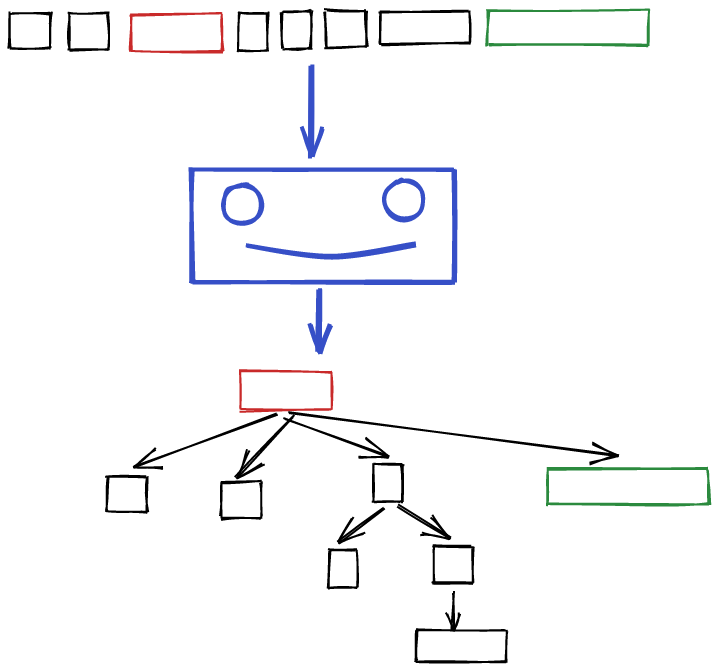
The goal of parsing is to go from our source code, to a representation that we
can actually work with. We want to transform Haskell code like:
foo = 2 + 3 * 4
into some kind of data structure that we can progressively
analyze and transform into C code. We’ll need to analyze things
like the scoping of names, and the usage of types. We’ll also
be gradually transforming and simplifying our representation,
with the goal of getting closer and closer to C.
We’ve already written one chunk of this parsing: the lexer.
The lexer takes some source code, and groups it up into small tokens.
Each token doesn’t
make sense as separate chunks. Our parser needs to take these tokens,
analyze their structure, and produce a data structure representing the source code.
More than Tokens?
Our lexer already gives us a data structure: a list of tokens. Why not just use
this to represent Haskell code?
Unfortunately, this isn’t going to work;
the tokens aren’t expressive enough to really reflect the structure
of Haskell.
Take this example:
x = 2 + 2y = 2
After lexing, we get a flat stream of tokens:
{ x = 2 + 2 ; y = 2 }
But this flat representation fails to capture the nested
nature of this snippet.
A better representation would be something like:
((x = (2 + 2))(y = 2))
The expression 2 + 2 “belongs” to the definition of x, and the expression
2 “belongs” to the definition of y. This kind of nested structure
is ubiquitous throughout Haskell. A list of tokens
is simply a bad fit here.
Trees
On the other hand, this kind of nesting is perfect for a tree.
Let’s take our previous example once more:
x = 2 + 2y = 2
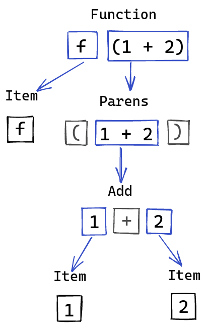
This piece of code can be represented by a tree that looks something like this:
Each node in the tree has some kind of label, and can contain other subtrees as children.
We have a node at the top level, containing all the top level definitions.
Definitions
use an = here, have the name as one child, and the expression as the other.
Addition uses a + node, with its arguments as children.
This approach scales nicely to expressions with even more nesting:
x =
  let y = 2 + 2
  in y
We now have a two nested expressions for x, giving us a tree that looks like:
We can imagine how this might work for even more complicated expressions, since
nodes can contain arbitrary trees as their children.
Valid Syntax vs Valid Semantics
This tree of nodes built up from source code is called an Abstract Syntax Tree, or
an AST, for short. It’s a syntax tree, since it represents the structure of
our programming language: what syntax is valid or not. I don’t actually know why
it’s called an abstract tree, but I like to think that it’s abstract, because it provides
a representation of trees that are syntactically valid, but that don’t necessarily make any sense.
For example, take this snippet:
x =
  let y = "34" + 3
  in "x" foo
This bit of code is syntactically valid, and our parser shouldn’t complain.
It still has a few issues though:
You can’t add strings and numbers
You can’t use a string like "x" as a function
The name foo is not defined in this scope
Because of these issues, our program is semantically invalid, even though it manages to parse.
The goal of the type checker is to find all of these issues. We’ll get to this
soon enough, but not in this part.
It’s not our parser’s job to figure these things out yet. Our parser is just concerned
with producing this Abstract Syntax Tree.
The parser will be taking the tokens produced by the lexer, and
transforming them into this tree.
Grammars
One common tool used to describe these syntax rules is a
Context Free Grammar,
or just Grammar for short. Grammars allow us to think about the structure
of a programming language, at least at the level of syntax.
As a motivating example, let’s take a very simplified subset of Haskell.
Our example language consists of a single expression, which might be one of:
A string literal:
"foo"
An int literal:
345
A variable name:
x3
Or, a let expression, with explicit braces and semicolons:
let { x = 3; y = 2;} in x
Note:
For simplicity, we require a semicolon after each definition,
instead of between them. This is slightly different than how we’ll handle
this in our real language, but is simpler for now.
A Grammar for this language would like something like this:
Each <rule> references some type of syntactic element. For example, <expr>
references
an expression in our little language. After the ::=, we declare each
way we can build up this element. Everything outside of angle brackets
is an actual token we expect to see.
For <expr>, this matches the overview we gave earlier: an expression is either
an integer literal, a string literal, a name, or a let expression.
And then, <letexpr> consists of the token let, followed by some definitions inside
braces, the token in, and an expression.
<definitions> is either empty, or a single definition followed by a ;,
and some more definitions.
Finally, <singleDefinition> represents things like x = 3.
This is just a name, the token =,
and then an expression.
Intuitively, this grammar allows describes the rules that define
what structure our toy language has. These kinds of rules should actually
be familiar for us, since our lexer used a similar approach.
For example, to define what a token was, we built
up a large lexer from smaller possibilities:
<token> ::= <keyword> | <operator> | <literal> | <name><keyword> ::= let | do | ......
The big difference is that our tokens were completely flat.
Tokens never contained
other tokens. Grammars, on the other hand,
allow us to talk about recursive structures as well.
Our toy language has a recursive structure: expressions can contain let
expressions, which also contain expressions. Because of this, you
can nest expressions inside of eachother:
let { x = 2} in let { y = x} in let { z = y} in z
Grammars should also seem eerily familiar to you as Haskeller. In Haskell, we
have algebraic data types.
For example, let’s define a type for colors.
A color can be either red, blue, green, or an arbitrary hex string like “#ABFE00”.
We could represent this with an ADT, like this:
data Color = Red | Blue | Green | Hex String
But, if you squint a bit, this looks kind of like a grammar:
We can go in the other direction, from grammar
to ADT, modelling this structure using Haskell types:
data Expr = IntExpr Int | StringExpr String | NameExpr Name | LetExpr [Definition] Exprdata Definition = Definition Name Expr
There’s not a one-to-one correspondance here, since the grammar is also concerned
with syntactic elements, like semicolons, and braces, and we don’t care about those
here. But the rough structure is the same, especially in terms of how the data type
references itself recursively.
Because Haskell has these nice recursive ADTs, we can
have our syntax tree look very similar to the grammar
for our language.
We won’t be using grammars directly, but we’ll be doing awfully similar things.
I also think it’s important
to touch on the concept of grammars, at least briefly, since most of the other resources
you’ll read about parsing will use them heavily.
Parser Combinators
Alright, now it’s time to start writing some code. Before we start defining the structure
of our syntax tree, or writing the parser itself, we first need to write our tool
of choice for making parsers: the Parser Combinator! This is going to be a suped up
version of the Lexer Combinator tool we made last time, extended to handle
recursive structures!
Let’s first create a module for our parser in our cabal file:
  exposed-modules:     Ourlude
                     , Lexer
                     , Parser
Now let’s go setup the standard module and imports in src/Parser.hs:
We have LambdaCase as a convenient extension in this module. We also import
Alternative, as well as some other utilities.
From Lexer Combinator to Parser Combinator
With Lexer Combinators, a lexer was essentially just a function:
input -> Maybe (a, input)
We take in some input,
and then either fail or succeed, returning a value, and the remaining input. This works well for lexing,
since a lexer can only produce one result,
and it’s always obvious which of two options we need to choose:
just use the longest match rule.
This won’t work for parsing. Our structure is much more complicated, so it’s not always
obvious that the longest match rule will be correct. What we do instead
is to let ambiguity happen, at least temporarily.
Instead of either failing, or returning a single way of consuming
the input, we return all possible ways to proceed forward.
We now have:
input -> [(a, input)]
By the time we’ve parsed the entire source code, there should be only a single element
in this list. Otherwise, there are multiple ways of parsing some code. For example,
a parser that doesn’t handle operator precedence might see 2 + 3 * 4 and produce both:
(2 + 3) * 42 + (3 * 4)
Of course, the second option is correct, because * has higher precedence than +, as we’ll
see later.
Ambiguity in the parsing process is fine, as long as we resolve it later. We might need more than
one token to resolve this ambiguity, which is ok. As a chief example, take where expressions.
These are expressions with the definitions coming after the body they’re used in:
x + y
  where
    x = 2
    y = 3
If in our parser for expressions, we have some rule like:
expr = notWhereExpr <|> whereExpr
Then we’ll have some ambiguity here. This is because we can’t tell which of these parsers is correct
until we see the where token. For the first 3 tokens,
we have multiple options floating around.
Note:
It’s possible to rearrange how you decompose your parser to avoid unbounded ambiguity
like this. For example, you could always parse an expression, and then change the meaning
of what you’ve just seen based on whether or not you see a where. We won’t be needing
these kinds of tricks, but they can make parsing more efficient.
By the time we finish parsing the file, we shouldn’t have any ambiguity left. If we do,
then that means that there are multiple ways of interpreting some code. This is basically
never a problem in the code itself, but a problem in the implementation of the language.
There are certain languages that are inherently ambiguous, like C++, in which case
the parser needs to make an arbitrary choice, but Haskell is not ambiguous. If we
fail to parse something because of ambiguity, that’s probably a bug in our parser.
The Concrete Type
With all of this in mind, we can go ahead and define a concrete type for Parser:
This is very similar to our Lexer type from the last part. Instead of working over String,
we know work over [Token], instead.
We also return multiple possible ways of parsing, as explained earlier.
Example Building Blocks
To learn how this works better, let’s go ahead and make a couple basic
helpers.
First, let’s make a little helper that accepts a single token:
satisfies :: (Token -> Bool) -> Parser Tokensatisfies p = Parser <| \case t : ts | p t -> [(t, ts)] _ -> []
This is analogous to Lexer.satisfies, which accepted a single character.
Our implementation looks at the remaining list of tokens,
and checks if there is a token matching our predicate
at the front of the list.
If so, we return that token, along with the remaining input. Otherwise
we return an empty list, since there’s no way for this parser to succeed.
An immediate application of this satisfies function is going to be:
This just matches against a specific token that we provide.
A similar function to satisfies is going to be pluck:
pluck :: (Token -> Maybe a) -> Parser a
The behavior is going to be the same as satisfies, except now we
can return a value
if the predicate matches. This is useful, because we have a few tokens like
IntLit i and StringLit s which also have an argument. This helper
lets us match against a token like this, extracting the argument. For example, we can do:
pluck <| \case
  IntLit i -> Just i
  _ -> Nothing
to get a parser that accepts an int literal, but produces an Int.
The implementation of pluck is similar to satisfies:
pluck :: (Token -> Maybe a) -> Parser apluck f = Parser <| \case t : ts -> case f t of Just res -> [(res, ts)] _ -> [] _ -> []
Just replaces the True case we had previously, but also provides
us with the value we want to return.
Functor and Applicative
Like with Lexer, we’ll be providing instances of Functor and Applicative
for Parser.
For Functor, we have:
instance Functor Parser where
  fmap f (Parser p) = Parser (p >>> fmap (first f))
This just maps over the results that we’ve produced. In fact,
this definition is exactly the same as for Lexer, since Maybe
and [] are both Functors!
For Applicative, the operations will mean the same thing as
for Lexer. pure :: a -> Parser a will give us a parser that always succeeds,
consuming no input, and (<*>) :: Parser (a -> b) -> Parser a -> Parser b will
give us a parser that runs the first parser, and then runs the second parser.
The return value will be the function
produced by the first with the argument produced by the second.
The difference with Lexer is that now a parser may return multiple results.
We’re going to use all the combinations of first and second results:
instance Applicative Parser where
  pure a = Parser (\input -> [(a, input)])
  Parser pF <*> Parser pA =
    Parser <| \input -> do
      (f, rest) <- pF input
      (a, s) <- pA rest
      return (f a, s)
pure does exactly what we said it does before, so it’s not too surprising.
What’s neat with <*> is that to implement the “combine all possible functions and arguments”
behavior,
we can use the fact that [] implements the Monad class in the same way that Maybe does,
allowing us to use do notation. For [], instead of allowing us to handle failure,
we are now able to handle “non-determinism”. What ends up happening is
that for each possible pair (f, rest) of a function, and remaining input,
we return each possible way of using the second parser on that input, and then
applying the function on the argument produced.
In practice, most of the time there won’t be any ambiguity, so:
parser1 *> parser2
will simply mean “run parser1, and then run parser2”
then we’ll get 2 * 2 = 4 paths available to us. We can parse 1A and then 2A,
1A and then 2B, etc.
Alternative
As you might expect, we’ll also be implementing Alternative for Parser,
to get that sweet sweet <|> operator, and all the goodies that come along with it!
We also need an empty :: Parser a function, which returns a Parser that always fails.
instance Alternative Parser where
  empty = Parser (const [])
  Parser pA <|> Parser pB =
    Parser <| \input -> pA input ++ pB input
To get a parser that always fails, we return no valid ways
to continue parsing.
For <|>, we run both parsers, and then combine both of their results using ++.
Unlike Lexer, we don’t try to resolve any ambiguity if they both succeed.
As explained earlier, we let the ambiguity exist, by returning all possible
ways of parsing. Our final parser should only end up returning one result though,
even if sub-parsers might temporarily have some ambiguity.
Like last time, the Alternative instance gives us plenty of goodies for free.
For example, we now have many :: Parser a -> Parser [a], which allows
to turn a parser for one item, into a parser for many items, placed one after the other.
There’s also some, which does the same thing, but requires at least one
item.
For example, if intParser accepts 3, then some intParser would accept 3 4 5 6, producing
[3, 4, 5, 6] as our output.
Integrating a Parser
We now have the combinators we need to build our parser. Before we
actually start working on parsing our subset of Haskell, let’s go ahead
and add a new stage to our compiler. We can get all of this boilerplate
out of the way, letting us focus on parsing.
Let’s define a stub type for our syntax tree, and for our errors:
Like last time, we just have a single error: the error telling
users that our parser is not implemented yet!
Our AST is just a stub data type as well.
We’ll be completing both of these soon enough. For now, we just want
to get this stage of the compiler integrated into the command line program.
We also need to write a simple parser function that we can expose
as our implementation of this stage:
parser :: [Token] -> Either ParseError ASTparser _ = Left UnimplementedError
This function will take in the list of tokens produced by the lexer,
and return either the parsed syntax tree, or an error, indicating
that parsing failed.
Finally, we can add the AST type and the parser function to the the
exports for this module:
module Parser (AST(..), parser)
Note:
Right now, we don’t need to export the constructors of AST in order
to make the stage. The stages we’ll add in the next parts will be working
with the details of the syntax tree, so we’ll need to export
its constructors, as well as the other data types we’ll add in this part.
Adding a new Stage
We now need to go into Main.hs, and add a Stage for the parser. First,
let’s add the Parser module to our list of imports.
-- ...import qualified Parser-- ...
Right next to lexerStage, we can go ahead and add a new Stage for our parser:
The definition of this is essentially the same as we had for lexerStage.
Stages were introduced in great detail
last time,
so feel free to take a quick refresher if you’d like.
We also need to modify our argument parsing to accept “parse” as a stage.
This way, users can do:
haskell-in-haskell parse file.hs
in order to print out the AST they get from parsing file.hs.
Of course, they’ll still be able to do:
haskell-in-haskell lex file.hs
to just print out the tokens they get after lexing file.hs.
Here we get to use the fancy >-> operator we defined last time, in order
to compose the lexing stage with the parsing stage. This works out nicely,
since the parsing stage consumes the tokens that the lexing stage produced.
We end up with a stage taking in a String for the source code,
and producing the AST that we want to print out.
We can now run all of this, and see something like:
> cabal run haskell-in-haskell -- parse foo.hsParser Error:UnimplementedError
which makes sense, since we haven’t implemented the parser yet. Let’s
fix that!
Structure of the AST
Before we can write a parser to convert our tokens into a syntax
tree, we need to define the shape of that syntax tree.
We’re going to be describing the exact subset of Haskell
that we implement, by creating various data types for each construct
in the language.
For example, we’re going to have a data type for expressions. One of
the variants will be a binary expression, for things like 1 + 2,
or 4 * 33. Another variant might be function application, for things like
f 1 2 x. etc.
A Rough Idea
Our subset of Haskell is almost cleaved into two distinct parts:
The part of the language dealing with defining types
The part of the language dealing with defining values
These 2 parts interact through annotations, which allow
us to declare that a given value has a certain type.
For example, if you have:
x :: Int -> Intx = \x -> x + 1
The Int -> Int is squarely in the domain of types, and we’ll need some data structures
to describe function types like Int -> Int. The lamdba expression \x -> x + 1 is clearly
in the domain of values. And the declaration x :: ... is a point of interaction
between both domains.
Because of this, we can think of our language as being roughly groupable
into 3 sections:
Definitions: assigning types and expressions to names
There’s a lot of interaction between these categories of course. For example,
let x = 3 in x is an expression that also uses a definition, inside
of the let. With that said, it’s still useful to have a bit of categorization
in our head before we start defining everything we need.
Types
So, the first thing we can do is define how we’ll work with types in this subset
of Haskell. We need ways to refer to certain types, like Int, String.
We also need to be able to use more complicated types,
like (Int -> String) -> String. We’ll
need ways to define new types, either through custom types, like
data Color = Red | Blue | Green, or type synonyms, like type MyInt = Int.
The Fundamental types
Before we get to the definitions of new types, let’s first define our data structures
representing types that exist. For example,
when you have x :: Int -> Int, you need some way of representing the
type that comes after the ::. This is what we’ll be defining now.
Essentially, what we’re doing is defining what a type “is” in our subset of Haskell.
In fact, this definition will be useful beyond just parsing. We can also use
this representation of types in our type checker, for example. Because of this,
we won’t be creating this definition of what at type is in the Parser module,
but instead creating a new module, in src/Types.hs, to hold fundamental data
structures for working with types. We’ll expand on this module in further parts,
as we need to do more things with types.
Note:
There’s an argument to be made for never sharing things like this between different
stages. It might be more maintainable to distinguish between the syntax of what
constitutes a type, and the semantics of what a type really is. Essentially,
the difference is that the former talks about what things the user can type in their
source code to tell your compiler about types, but the latter defines how the compiler
itself manipulates types.
For example, this approach allows you to add syntax sugar for different types:
maybe A <-> B is syntax sugar for (A -> B, B -> A) in your language. Your representation
of types later on doesn’t have to deal with this extra construction, if you separate
the syntactic types from the “actual” types.
We won’t be using a separation like this for our types, but we will have
a simplifier phase for expressions. We’ll be going over this phase in the next post.
It just turns out that for types, there’s not really anything we can simplify,
so it’s a bit more convenient to not bother with the extra boilerplate of having
two isomorphic representations.
As usual, let’s edit our .cabal file to add the Types module:
  exposed-modules:     Ourlude
                     , ...
                     , Types
Now, we can go ahead and define this module in src/Types.hs:
module Types whereimport Ourlude
For now, we just export everything in the module, but we’ll come back and make the
imports explicit once we’ve defined our representation of types.
First, let’s think about what kind of types you should be able to work with in
our subset of Haskell. As mentioned already, we’re going to have a primitive
Int type, the standard integer type we’re used to.
Integer literals will have that type, so 3 :: Int, for example. We’ve already
lost the element of surprise by defining boolean and string literals in the lexer,
so we’re going to also have primitive boolean and string types in
our language, departing from Haskell slightly.
So we have String and Bool as builtin types as well.
Note:
Our subset of Haskell would be expressive enough to define these in the language itself:
The reason I’ve opted to make these primitive instead is that to do this thing well,
you need some kind of module system, which is out of the scope for the subset
we’re trying to make with this series.
In addition to builtin types, we need a way for users to define new types,
and then reference those types. If a user has type X = Int, then
they should be able to say:
y :: Xy = 3
So we need to reference custom types by name, as well.
Our subset will also have support for polymorphism. You can define functions like:
id x = x
The type of this function is polymorphic:
id :: a -> a
Here, a is not a type per se, but rather a type variable. We need a way
to reference type variables by name as well.
This also means that custom data types can be polymorphic, and have variables of their
own. For example, you might define a list data type as:
data List a = Cons a (List a) | Nil
This will be valid in our language, and introduces the type List _, where the underscore
needs to be filled in. So you might have List Int as one type,
List String as another, and List a, if a happens to be a type variable in scope.
In brief, custom types are referenced by name, and also have multiple type variables
as arguments.
Finally, we need a way to talk about the function type A -> B, which is also
built into the language.
With all of this in mind, let’s just define our representation of types:
type TypeVar = Stringtype TypeName = Stringinfixr 2 :->data Type = StringT | IntT | BoolT | CustomType TypeName [Type] | TVar TypeVar | Type :-> Type deriving (Eq, Show)
So, we have the basic primitive types as hardcoded options:
Int corresponds to IntT in this representation
String corresponds to StringT
Bool corresponds to BoolT
We have 2 type synonyms, to clarify the difference between TypeVar, which is a lower
case name, like a, used for the name of a type variable, and TypeName, which
is an upper case name, like List or Foo, used to reference the name
of a newly defined type.
Type variables have the variant TVar and take a name as argument. So a in Haskell
would be TVar "a" in our representation.
For newly defined types, we have the name of that type, as well as a list of arguments,
which are also types. List Int would be CustomType "List" [IntT] in this representation.
You can also nest things, so List (List Int) would become
CustomType "List" [CustomType "List" [IntT]]
Note that type synonyms are also under this category. If you have type X = Int,
then you’d use CustomType "X" [] to refer to this type synonym.
Finally, we need a way to represent function types. We create a new operator
:-> for this. (We need the : so that it can be used in types). With this in place
Int -> Int becomes IntT :-> IntT, as expected. Note that we declare
this operator infixr, which means it’s right associative, like -> is in Haskell.
This means that:
Int :-> StringT :-> BoolT
is parsed by GHC as:
Int :-> (StringT :-> BoolT)
which is exactly the behavior that we want.
We’ll be using this representation of types throughout the compiler. Let’s go ahead and
explicitly export it as well:
module Types ( Type (..), TypeVar, TypeName )where
Now, let’s use these types to start working on our syntax tree, back in src/Parser.hs.
Defining new types
The next thing we need to do is add the data structures representing the definitions
of new types in our language. There are going to be two ways to define new types:
Type Synonyms, things like type X = Int
Data Definitions, things like data Animal = Cat | Dog
In our language, these are both considered as a kind of definitions
that can appear at the top level. They’ll both be variants of a common
Definition type.
We’ll be needing the items we just defined in the Types module inside of the parser,
so let’s add an import in src/Parser.hs:
First, let’s define type synonyms.
Note that we don’t allow polymorphic things like type List2 a = List a,
only type ListInt = List Int. Because of this, we can define type synonyms
as a simple variant of Definition:
data Definition
  = TypeSynonym TypeName Type
A type synonym has a name, which is an upper case name like X, and a type that
it’s equal to.
And then, we need to define the structure of data definitions. The basic idea
is that we have a name and some list of constructors:
data MyType = VariantA | VariantB | VariantC
We also need the ability to have arguments in each of the constructors:
data MyType = VariantA String | VariantB Int Int | VariantC
We can also make the data type polymorphic, by specifying some type variables
next to the name:
data MyType a b = VariantA String | VariantB Int Int | VariantC
Of course, we can use these type variables inside of the variants:
data MyType a b = VariantA String | VariantB Int Int | VariantC a b
And that’s about it for new data types.
Note:
Syntactically speaking, nothing is stopping us from using type variables that aren’t
even in scope, so something like data Foo = Foo a b c will parse just fine.
Of course, this makes no sense semantically, and will be caught by later stages.
Let’s first define a structure for each of the constructors / variants:
A constructor has a given name, like VariantA, or Cons, as well as a list
of types, which are the arguments for the constructor. For clarity,
we’ve created a separate synonym, ConstructorName, for this kind of name. For example,
the VariantB constructor in our MyType example would be represented as:
ConstructorDefinition "VariantB" [IntT, IntT]
Now, we can add an extra variant in Definition for data definitions:
data Definition
  = DataDefinition TypeName [TypeVar] [ConstructorDefinition]
  | TypeSynonym TypeName Type
  deriving (Eq, Show)
A data definition has a name, a list of type variables, and then a list of constructors.
Our MyType example becomes:
And now we have a complete way of representing the syntax for defining new types!
We’ve already started getting a feel for the tree like structure we’re using
to represent our language, and we’re just getting started!
Expressions
In this section, we’ll be defining most of the different kinds of expressions in our language,
except for let and where expressions. These will use definitions, which we’ll define
a bit later.
Literals
This first expressions we have are literals. We have int literals,
like 2 and 245, string literals, like "foo" and "bar", and finally,
boolean literals, namely, True and False. We can define a type Literal
representing these:
data Literal
  = IntLiteral Int
  | StringLiteral String
  | BoolLiteral Bool
  deriving (Eq, Ord, Show)
We have one type of literal for each of the primitive types in our language.
Let’s also add a type of expression for literals:
data Expr
  = LitExpr Literal
  deriving (Eq, Show)
As an example, the literal 3 becomes the much more verbose:
LitExpr (IntLiteral 3)
Names
We can also reference names inside of expressions. For example, if
we have some value x :: Int, we have x + x as an expression. We can also reference
the constructors for different data types, like Nil, Red, etc.
We’ll be representing these names with strings, but for clarity, let’s create a
type synonym:
type Name = String
We can then use it to define a kind of expression that just use a name:
data Expr
  ...
  | NameExpr Name
Semantically, the meaning of NameExpr "foo" is whatever expression
"foo" is bound to in a given scope. So if we have foo = 3, then
NameExpr "foo" should evaluate to IntLiteral 3, using our expression syntax.
If Expressions
Next we have if expressions, things like:
if y then 3 else 4if 2 + 3 > 4 then 4 else x + x
These are straightforwardly defined as:
data Expr
  ...
  | IfExpr Expr Expr Expr
We can have arbitrary expressions inside of the condition, if-branch,
and else-branch.
The next kind of expression are lambda expressions, allowing us
to define anonymous functions. These look like:
\x -> x + 1\x -> \y -> x + y
Note that in Haskell, you can define multiple names at once in a lambda. For example:
\x y -> x + y
is valid, and syntax sugar for:
\x -> y -> x + y
The simplifier will deal with this syntax sugar; our parser will accept this
verbatim:
data Expr
  ...
  | LambdaExpr [ValName] Expr
We have a list of named parameters, and then an arbitrary expression using them.
So \x y -> x becomes:
LambdaExpr ["x", "y"] (NameExpr "x")
This is the first time we use the ValName synonym, which is defined as:
type ValName = String
This will be used in many places for names that exclusively refer to values.
So x is a ValName, but something like Nil would rather be typed
as ConstructorName.
Note:
Since we’re using type synonyms here, there’s actually no difference between ValName
and ConstructorName. We could’ve used newtype instead, to make it impossible
to confuse them. The problem is that there are situations, like NameExpr,
where both might be valid.
For simplicity I’ve opted to not add the boilerplate of creating explicit differences.
The synonyms are mainly there for documentation, not correctness.
Function Application
What would our functional language be without function application? In Haskell,
function application just takes arguments separated by whitespace:
f 1 2 3
We can also have some arbitrary expression as the function as well:
(f . g) 1 2
This gives us:
data Expr
  ...
  | ApplyExpr Expr [Expr]
Because of currying, f 1 2 is really sugar for (f 1) 2. But, once
again, we’ll be removing syntax sugar in the simplifier; the parser
needs to accept all of this. So, for now, f 1 2 would be represented as:
We have a single unary operator in our language: negation. Instead of
having negative numbers, like -3, this is instead the negation operator
- applied to the expression 3. We can also do more complicated things like:
-((\x -> x + 1) 3)
So, we add negation expressions:
data Expr
  ...
  | NegateExpr Expr
This makes the simple -3 into the much more verbose:
NegateExpr (LitExpr (IntLiteral 3))
Binary Operators
With the only unary operator in the language out of the way, let’s add the
many binary operators we need. This will cover arithmetic like a + b + c,
to function composition f . g . h, to comparisons with x > y, etc.
We have:
data Expr
  ...
  | BinExpr BinOp Expr Expr
If we have some complex arithmetic expression, like a + a + b * (x + y), this can
still be written as a tree, with each node only having two children:
Of course, we haven’t defined Add or Mul, or any of the other members
of BinOp yet. Let’s briefly go over all of the operators:
data BinOp
  = ...
  deriving (Eq, Show)
The + operator is used to add two numbers:
= Add
The - operator subtracts the right number from the left number:
| Sub
The * operator is for multiplication:
| Mul
The / operator is for division:
| Div
We have ++ for string concatenation
| Concat
We have the comparision operators <, <=, >, >=, which become:
  | Less
  | LessEqual
  | Greater
  | GreaterEqual
And the comparison operators == and /= become:
  | EqualTo
  | NotEqualTo
We also have the two boolean operators ||, and &&, which are:
  | Or
  | And
Finally, we have the function “operators”. Namely, $ and .. These are defined
as standard functions in normal Haskell, but since we don’t have custom operators,
these are done here as well:
  | Cash
  | Compose
Note:
I have no idea how widespread calling the $ operator “cash” is. I’ve always
called it that since I first learned Haskell ~ 4 years ago. I’ve heard f $ x
read as “f dollar x”, but that doesn’t roll off the tongue like “f cash x” does.
Pattern Matching
The next kind of expression we’re going to deal with are case expressions, things
like:
case x of
  2 -> x + 2
  3 -> x + 3
  y -> x + y
or
case x of
  Nil -> 0
  Cons A (Cons B Nil) -> 1
  Cons B Nil -> 2
  Cons y Nil -> y
We have some kind of expression that we’re scrutinizing, followed by
a series of branches. Each branch has some kind of pattern that we’re matching
against, followed by an expression. The value of the case expression is the value
of whatever branch happens to match.
So, let’s first define what kind of patterns we have in our language:
data Pattern
  = ...
  deriving (Eq, Show)
The first kind of pattern is the wildcard: _. This pattern matches against everything,
but creates no new name:
data Pattern
  = WildcardPattern
The next kind of pattern is similar. We can also have a name as a pattern, like:
case 3 of
  x -> x
This is like the wildcard, but also assigns the value of whatever it managed to
match to the given name. Here, x would have the value 3 inside of the branch.
We have:
data Pattern
  ...
  | NamePattern ValName
We use ValName, since only lower case names like x are valid here.
Another kind of pattern is for literals. We can match against literal ints, like
3, literal strings, like "foo", or literal bools, like True, or False:
data Pattern
  ...
  | LiteralPattern Literal
We also want to be able to match against custom types. If we define a custom
type like data Color = Red | Blue | Green, we need to be able to do things like:
case color of
  Red -> ...
  Blue -> ...
  Green -> ...
If our data type has constructors, like data Pair = Pair Int String,
we want to be able to match against the arguments as well, giving us constructions like:
case pair of
  Pair 3 "foo" -> ...
  Pair x "bar" -> ...
  Pair _ _ -> ...
With this in mind, we need to add a variant for these constructor patterns:
data Pattern
  ...
  | ConstructorPattern ConstructorName [Pattern]
We have the name of the constructor, followed by a sequence of arbitrarily complex
patterns. So, given a data type like data List a = Cons a (List a) | Nil,
and a pattern like:
And now that we’ve defined patterns, we can immediately define case expressions!
data Expr
  ...
  | CaseExpr Expr [(Pattern, Expr)]
We first have the expression we’re scrutinizing, followed by a list
of branches. Each branch contains a pattern,
and the expression to use when that pattern matches.
Now that we’ve defined expressions as well as the structure of types,
we can combine the two, in order to define the structure of value definitions.
This is about the structure of defining new values. In Haskell, there are two parts
to a value definition:
The type annotation, like x :: Int
The name definition itself, like x = 3
The type annotation and name definition don’t have to appear together, and the
type annotation isn’t necessary at all. Regardless, our parser will need to represent
both.
We’ve just introduced the notion of a ValueDefinition, which will contain both
the type annotations, and the name definitions we’ve just touched upon. We’ve also
added this to our concept of Definition. A definition now includes the two
constructs related to types, namely, data definitions, and type synoyms,
as well as the definitions for values.
For type annotations, the definition is pretty simple:
data ValueDefinition
  = TypeAnnotation ValName Type
A type annotation like x :: Int is represented as the name of the value being annotated,
and the type we’re providing after the ::.
For name definitions, our first try might be something like:
NameDefinition ValName Expr
The idea is that something like x = 3 would become:
NameDefinition "x" (LitExpr (IntLiteral 3))
This would work for a large class of Haskell definitions, but Haskell
has some more syntax sugar around definitions. The first piece of sugar is that
instead of having to write:
id = \x -> x
You can instead move the parameter x to the left side of the =:
id x = x
Of course, you can have multiple parameters as well:
f a b = a + b
So, our structure for name definitions will need to accomodate these named parameters.
Another bit of sugar is that you can pattern match inside of these definitions:
f 0 1 = 1f 0 _ = 2f a b = a + b
A function can be defined with multiple “heads”, each of which has patterns for
its arguments. Because of this, our full structure for name definitions
becomes:
data ValueDefinition
  ...
  | NameDefinition ValName [Pattern] Expr
We have the name used for this value, a list of patterns for each of the arguments,
and an expression for the body of this definition.
We have one definition for the type annotation, and 2 more for each of the
2 heads of the function.
Note:
Note that we don’t even do any basic integrity checks for these heads,
like making sure that they have the same number of patterns. This kind of thing is going
to be handled in the simplifier.
Now that we have a structure for definitions, we can add the two missing
types of expressions: let and where expressions. These are
really two ways to express
the same thing: local definitions inside an expression. So:
let x :: Int x = 2in x
and
xwhere x :: Int x = 2
Have exactly the same meaning. For clarity, we’ll just create two different
types of expression for each of these:
The structure is slightly different, to reflect the different order of the two
variants. let has the definitions before the expression, and where has
the definitions after the expression.
Note:
We could’ve chosen to parse where as a let expression, or vice-versa,
but I like the clarity of representing the syntax exactly. As you might have guessed,
our simplifier will remove this redundancy.
Finally, now that we have definitions finished, we can actually
define our real syntax tree:
The next step
in this post is to write a parser for our AST, using the little combinator
framework we created earlier.
Parsing in Practice
So, now it’s time to use all of the little tools we’ve made
in order to build up a parser for our AST. We’re going to be building up a parser
in a bottom up fashion, starting with simple parsers for simple parts
of the language, and combining them piece by piece to make up a parser for the whole language.
Names and Literals
We’re going to be starting with the simplest form of expression: names,
and literals. There were two types of names in the lexer: LowerName,
for names starting with a lower case letter, and UpperName for names
starting with an upper case letter. We can make a parser for LowerName
pretty easily:
lowerName :: Parser ValNamelowerName = pluck <| \case LowerName n -> Just n _ -> Nothing
Here we use the pluck :: (Token -> Maybe a) -> Parser a function we defined previously.
pluck lets us match against a certain type of token, and also extract some information
about that token. This is useful here, since we want to extract
the string contained in a LowerName token.
We can use the same trick for UpperName:
upperName :: Parser TypeNameupperName = pluck <| \case UpperName n -> Just n _ -> Nothing
The only difference here is that we’re extracting from UpperName instead
of LowerName.
We’ve created a few different synonyms for String, to clarify the different
kinds of names we use throughout our AST: things like
TypeVar, TypeName, ValName, etc. We can immediately put the two parsers
we’ve just defined to use, by creating a parser for each of these syntactic
classes:
Each of these kinds of name is either a lower case name, or an upper case name. In some contexts,
for example, function application, we might need to accept both,
which is why we created the Name synonym. We can add a parser for that as well:
name :: Parser Namename = valName <|> constructorName
Here we use the <|> for the first time, to indicate that name
is either a valName, or a constructorName, i.e. that we should accept either
the LowerName token, or the UpperName token here.
The next thing we can add in this section is literals. We want to be able
to parse ints, strings and bools, which make up the built-in values in our
subset of Haskell:
Once again, we use the handy <|> operator, to say that a literal is either
an integer literal, a string literal, or a bool literal. The lexer has already
done the job of creating a token for each of these, which
makes defining these alternatives very easy:
  where
    intLit =
      pluck <| \case
        IntLit i -> Just (IntLiteral i)
        _ -> Nothing
    stringLit =
      pluck <| \case
        StringLit s -> Just (StringLiteral s)
        _ -> Nothing
    boolLit =
      pluck <| \case
        BoolLit b -> Just (BoolLiteral b)
        _ -> Nothing
We use the very handy pluck once again, in order to match against
the right kind of literal token, and pick out the data it contains. We then
make sure to wrap this data in the right kind of literal for our AST.
Int literals become IntLiteral i, strings StringLiteral s, bools BoolLiteral b,
as we went over before.
Parsing Operators
The next thing we’ll add support for is parsing operators.
This requires a bit of thought before we get to writing out our parser though.
Operator Precedence
A first approach
towards operators would be to treat them as a kind of punctuation. If you have something
like:
x + y - a + 3
The names and literals are like words composing this arithmetic sentence,
and the arithmetic operators
are like the punctuation between the words. A first approach would start with some parser
for these bottom level words. Then you’d use this parser, separated by the arithmetic
tokens:
One problem with this approach is precedence. For example, multiplication with
* has higher precedence than addition with +. This means that an expression like:
1 + 2 * 3 + 3 * 5
should parse as:
((1 + (2 * 3)) + 3) * 5
and not:
((((1 + 2) * 3) + 3) * 5)
We would get the latter if we parsed addition and multiplication with the same precedence.
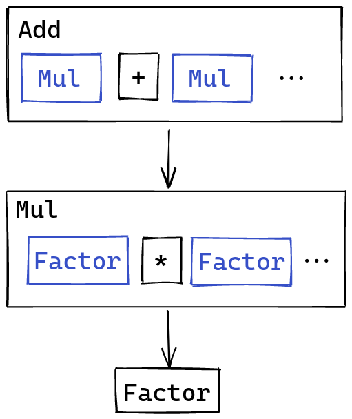
One way to fix this is to introduce
multiple layers, with one layer for each level of precedence:
Addition would parse multiplication, separated by +, and multiplication would
parse literal factors, separated by *. This paradigm allows us to skip
levels too. A single item like 3 falls under the “at least one number separated by *”
category: we just have the single number.
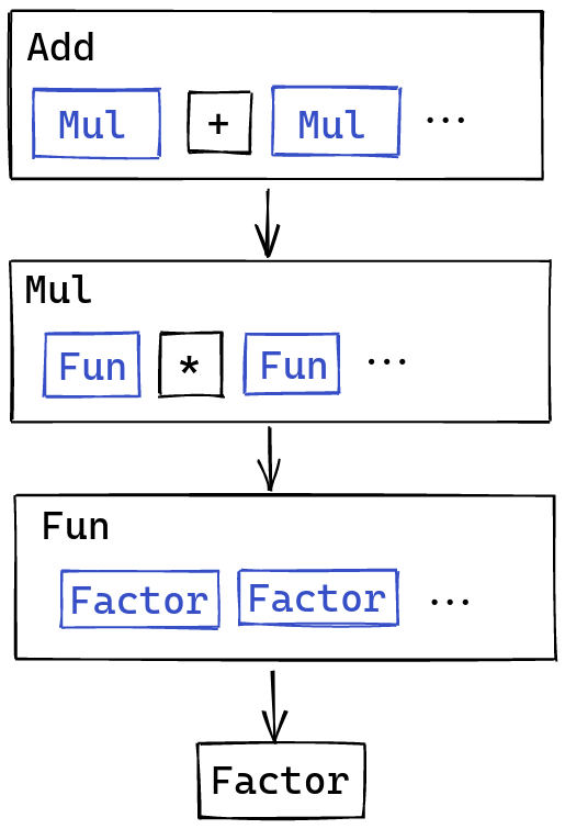
Function application falls under this paradigm as well. We can treate
function application as a very high precedence kind of operator. Instead of
parsing “at least one <sub-factor>, separated by <operator>”, we just parse
“at least two <sub-factor>s”. (This makes sure that,
only f x is considered as a function application, since f alone
would just be a name).
With multiplication, addition, and function application, our tower of operators
now looks like this:
One aspect is missing though: parentheses! In languages with arithmetic expressions like
these, you can manually insert parentheses to override the grouping rules.
For example, this expression:
(1 + 2) * 3
is not the same thing as:
1 + 2 * 3
precisely because the parentheses have been inserted.
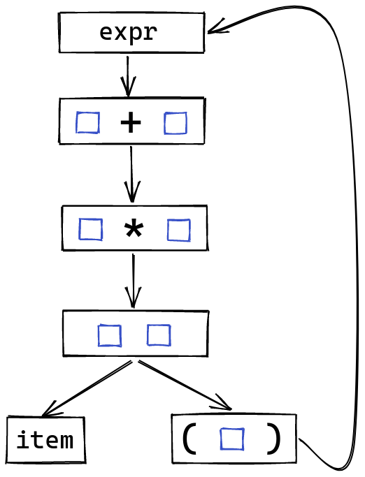
There’s a simple rule to make this work. Instead of having the bottom of our tower
only have dead-end rules like literals, or simple names, we can instead add
a rule that goes all the way to the top, parsing any expression surrounded with
parentheses:
Parsing some expression like f (1 + 2) will work, because we end up with a transition
like this:
This is also useful beyond arithmetic, since we wanted to allow arbitrary expressions
inside of parentheses anyways. As bizarre as it may seem, something like:
function ( case x of 1 -> 2 _ -> 3)
is a valid bit of Haskell. This precedence looping trick will allow us to parse
this kind of thing once we expand our expressions to accept more than
just operators.
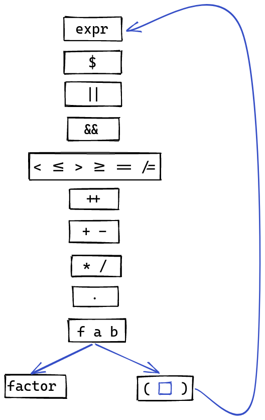
Using this approach, a full precedence tower including
all of the operators in our language looks like this:
(See this link
for a good overview of the precedence of different operators).
With that in mind, have enough thinking done to start implementing this precedence tower.
Operator Utilities
The parsing for each layer of operator will be very similar, so we can go ahead
and define a handful of utilities we’ll be using to build them up.
The first utility is to take a parser for <item> and turn it
into a parser for ( <item> ). This is useful for implementing the looping
in our tower of precedence. This utility just requires matching
() tokens before and after the original parser:
parensed :: Parser a -> Parser aparensed p = token OpenParens *> p <* token CloseParens
Here we use the convenient *> and <* operators:
(*>) :: Applicative f => f a -> f b -> f b(<*) :: Applicative f => f a -> f b -> f a
These sequence their arguments in the same order as <*>, but pick a different
result. For our parensed parser, this does the right thing, parsing
the ( before our original parser, and the ) after, but leaving us with
just the original result.
When thinking about parsing operators, we had the nice of idea of doing
something like “parse at least one factor, separated by an operator”.
We can make a utility that does this:
sepBy1 :: Parser a -> Parser sep -> Parser [a]
Given a parser for a, and parser for sep, this creates a parser that
parses one or more occurrences of a, separated by sep. So,
something like sepBy1 literal (token Semicolon) would parse things like 3;1;"foo".
The implementation makes straightforward use of a few utilities for Alternative:
sepBy1 :: Parser a -> Parser sep -> Parser [a]sepBy1 p sep = liftA2 (:) p (many (sep *> p))
Semantically, we first parse p, and then zero or more occurrences of
sep followed by p. So:
<p><p> <sep> <p><p> <sep> <p> <sep> <p>
are all going to be accepted by this parser.
many :: Alternative f => f a -> f [a] is provided to us, since parsers
implement the Alternative class.
We use sep *> p each time, since we just want the item parsed, and not the separator.
Finally, we use liftA2 (:) to cons the first item parsed, with the many items
produced by the rest of the parser.
Now, this would work for something simple like multiplication, since we
could parse out many multiplication factors, separated by *. One slight
problem is that some operators have the same precedence. For example,
+ and -. We need a modified version of sepBy1 where we remember
the separators we see. In fact, it would be even more useful
if given something like:
1 + 2 - 3 + 4
our parser could recognize this as:
1 (+, 2) (-, 3) (+, 4)
and then build up the correct parse tree, using each operator:
((1 + 2) - 3) + 4
This inspires the following type for parsing operators:
opsL :: Parser (a -> a -> a) -> Parser a -> Parser a
The first parser is used for separators, and the second parser is used
for the factors between separators. Semantically, this acts
like sepBy1, with the arguments reversed. The key difference is that
our separator parser produces a function used to combine the items
to its left and right. For example, for parsing addition and subtraction,
we could use this as our separator:
If we see a +, we combine things as an addition expression, and if we see
a -, then we combine things with a subtraction expression.
The implementation is similar to sepBy1
opsL :: Parser (a -> a -> a) -> Parser a -> Parser aopsL sep p = liftA2 squash p (many (liftA2 (,) sep p)) where squash = foldl' (\acc (combine, a) -> combine acc a)
Instead of discarding the separators, we now keep them alongside
the tokens:
Then, we fold from the left, using the combinator that’s now attached
to each token we encounter:
In practice, this works out nicely. Given some arithmetic expression
like:
a + b + c - d
this groups things in the way we’d expect:
((a + b) + c) - d
One problem is that this works for left associative operators, since
we have our large expression on the left, and add items
as we scan towards the right.
Some operators are not left associative though! For example,
the function arrow -> between types associates to the right:
For example, this snippet:
Int -> String -> Int
means:
Int -> (String -> Int)
and not:
(Int -> String) -> Int
We need to create an opsR function, that does the same thing as opsL,
but associates to the right instead:
opsR :: Parser (a -> a -> a) -> Parser a -> Parser a
The idea is that given some sequence, like:
A -> B -> C -> D
We end up with:
after grouping the items and the separator, like we did in opsL.
Next, let’s flip this sequence around, before moving the separator
to the right one step:
Now we also need to flip
the operator, to make sure that the arguments are passed in the right order.
And then our scanning approach from last time works:
With this in mind, here’s the implementation of opsR:
opsR :: Parser (a -> a -> a) -> Parser a -> Parser aopsR sep p = liftA2 squash p (many (liftA2 (,) sep p)) where shift (oldStart, stack) (combine, a) = (a, (combine, oldStart) : stack) squash start annotated = let (start', annotated') = foldl' shift (start, []) annotated in foldl' (\acc (combine, a) -> combine a acc) start' annotated'
Our starting point is the same as with opsL, having parsed our
first item, and the following items along with their separators. From there,
we do a first scan, where we want to end up with each separator
attached to the item on its left, and the last item in our starting list
alone.
We do this with foldl', keeping track of the last item we’ve seen, and
the tail of items along with their new separators. When we see a new (sep, a)
pair, a becomes our new last item, and the previous item
is paired up with sep, and put onto the tail.
Finally, we can scan over this list as if we were doing a left associative
operator, with the caveat that we swap the arguments to combine.
This is because we need to apply flip combine in practice,
and not just combine, to accomplish the “operator flipping”
we went over in the previous diagram.
In practice, this means that if we have:
A -> B
which we’ve separated into:
(B, [(->, A)])
the -> function is still expecting the accumulator on its right,
to make, A -> B.
Note:
Of course, we could have swapped the convention for opsR, making it accept
the separator function in the same order in which it ends up using it, but
this would make things needlessly complicated for the consumer of this function.
This took me a while to get a hold of as well, but thinking through the illustrations
really helps make sense of how this operation works.
Operators in Practice
At the top of our precedence hierarchy, we have expressions:
expr :: Parser Exprexpr = binExpr
For now, all the expression we have are binary expressions. This is where we’ll
have all of our operator parsing.
Here we have different possibilities, since all of these operators have the same
precedence. For each of the possible tokens, we make sure to associate
the correct binary expression. Each operator parser
always yields exactly the combining function that it represents,
thanks to our use of <$.
Continuing on, we have ++, for string concatenation:
Next come unary operators, of which we only have -x, for integer negation.
Note that -(+1) 3 is valid haskell, and evaluates to -4. This still looks
a bit weird to me, but is pretty simple to handle:
To parse a unary expression, we either find a - and a function application expression,
or just skip the - entirely.
appExpr is going to parse something like f a b c, and decide whether
or not it’s a function, based on how many things it sees:
appExpr :: Parser ExprappExpr = some factor |> fmap extract where extract [] = error "appExpr: No elements produced after some" extract [e] = e extract (e : es) = ApplyExpr e es
If we see a single expression, then we leave that alone. Something like 3
by itself just means 3. If we see f 3, i.e. two or more items, then
the first of those items is a function, and the rest are its arguments.
Note:
The some function provided by Alternative parses one or more occurrences
of a parser, so if it produces an empty list, that’s not our fault,
and something very fishy is going on.
This is why some people advocate for more usage of the NonEmpty type in
Haskell, which would allow many and some to indicate how they differ
in terms of their types:
some :: f a -> f (NonEmpty a)many :: f a -> f [a]
And finally, we have factor, which is at the bottom of our precedence hierarchy:
A factor is either a simple literal, a name, or it pulls off the beautiful
trick we went over earlier: it expects some parentheses, and jumps
all the way back to the top of the expression hierarchy!
Other Expressions
The next thing we’re going to tackle is parsing expressions that don’t contain
definitions, i.e. if, case and lambdas.
If expressions and lambdas are pretty simple, so let’s get them out of the way:
    ifExpr =
      IfExpr
        <$> (token If *> expr)
        <*> (token Then *> expr)
        <*> (token Else *> expr)
We parse the condition after an if token, the first branch after
a then token, and the other branch after an else token. We use the standard
<$> and <*> operators to plumb these results into the IfExpr constructor,
which takes these three operands.
For lambdas, it’s also not that complicated. A lambda like:
\x y -> x + y
is just the \ token, some names, a -> token, and then an expression. In code,
we get:
For case expressions, we first need a way to parse patterns. Parsing
patterns is kind of similar to operators. We can have a constructor with simple
arguments:
C 1 2 3 4
but in order to introduce more complicated patterns as arguments, we need parentheses:
C (A 2) 2 3 B
Notice how the B constructor takes no arguments,
and can appear without as a simple argument here.
Our definition for a single pattern looks like this:
A pattern is either a constructor taking some arguments, or a single
argument pattern. unspacedPattern will parse any kind of pattern that can
appear as an argument to a constructor, perhaps requiring parentheses:
unspacedPattern :: Parser PatternunspacedPattern = simplePattern <|> parensed onePattern where
So, an unspacedPattern is either an entire pattern, wrapped in parentheses,
or a simple pattern, which can appear as an argument
without any parentheses:
A pattern like this is either a constructor with no arguments, like
B in the example before, a wildcard pattern _, a single named
pattern, like x, or a literal, like 3 or "foo".
With patterns defined, we can start working on case expressions. Note that
from the point of view of the parser, case expressions use braces and semicolons:
case x of { 1 -> 2; _ -> 3}
This kind of situation will appear with definitions as well, so we can go
ahead and make a utility for parsing braces and semicolons:
braced :: Parser a -> Parser [a]braced p = token OpenBrace *> sepBy1 p (token Semicolon) <* token CloseBrace
braced turns a parser for a single item, into a parser for one or more items
separated by semicolons, all inside of braces.
We can then immediately used braced to create a parser for case expressions:
We have the case <scrutinee> of part, followed by the patterns,
which are in braces and semicolons. We than have the <pat> -> <branch>
part. Each pattern is just the
onePattern we defined before, followed by the -> token,
and the expression for that branch.
We could add this to the definition of expr, but we’re going to be
adding a few more expressions shortly, so we can just include it when
we get around to those.
Types
The remaining expressions are those related to definitions:
things like x = 2, or x :: Int. We can parse the expression part
of these value definitions just fine, but we haven’t added any parsing
for types yet! We’ll take care of this now, before moving
on to definitions.
Parsing types is going to be very similar to parsing patterns.
We have some types taking in arguments, like Pair Int String,
or List (List Int). We need to distinguish the types
that are basic enough to appear as arguments without parentheses,
like we did with patterns.
We’ll also need to add in a bit of operator parsing, to parse
function types like Int -> String -> Int.
We have different type “factors”, separated by the function arrow ->. This
becomes the constructor :->, representing the same thing in our syntax tree.
Of course, we make sure that we parse this operator in a right associative
way, so that:
Int -> String -> Int
is parsed as:
IntT :-> (StringT :-> IntT)
The base type that can appear between functions is either the single type
we defined earlier, or a custom type, which we excluded from the definition
of singleType. A custom type is parsed as some type name, followed by zero
or more arguments.
For the arguments, we do something interesting. We accept singleType, as
expected, but we also accept namedType. namedType is just a single
custom type, without any arguments. This allows us to have
a type like T as an argument, giving us something like Pair T T,
without needing to wrap T in parentheses.
Note:
The reason we couldn’t have moved this case inside of singleType is
becase of ambiguity. If it were possible to parse something like T
by going through singleType, then it would also be possible
to parse it by going through customType, and having no arguments
coming from many. Because we have multiple ways of parsing, we would
end up with multiple results after running our parsers, which we
do not want.
Value Definitions
With that in place, we now have everything we need to parse value definitions.
As a reminder, these look like:
x :: Intx = 3
We have either a type annotation, or a name definition. The parser for
this is pretty straightforward:
A valueDefinition is either a nameDefinition, or a typeAnnotation.
A typeAnnotation is a name, followed by a :: and some type.
A nameDefinition is also a name, but this time with multiple patterns
as arguments, the = token, and then expression. We have multiple
patterns, since Haskell allows the syntax sugar:
f a b = a + b
for:
f = \a b -> a + b
These are unspacedPattern, since if we need complex patterns, we need them
to appear with parentheses. Something like:
f Pair a b =
will be parsed as:
f (Pair) (a) (b) =
instead of:
f (Pair a b) =
which requires explicit parentheses.
Remaining Expressions
With these value definitions in place, we’re now ready to finish defining all
of our expressions. The remaining expressions
we need to add to expr are where and let expressions:
It should be clear that notWhereExpr <|> whereExpr includes every
kind of expression, unless you’re a constructive mathematician.
For let expressions, we just parse the token let, followed by
some value definitions in braces and semicolons, the in token,
and then an expression.
Remember that let introduces a layout, so:
let x :: Int x = 2in x
is lingo for:
let { x :: Int; x = 2} in x
Now, for where expressions, it’s tempting to do something like:
expr *> token Where *> braced valueDefinition
but the problem is that this parser recurses infinitely. This is an issue
we haven’t touched upon yet, called left recursion. This arises
in theory for parsing methods like ours, and for parser combinators
in particular, even in a lazy language like Haskell.
The fundamental problem is that if we have a rule like this,
to parse expr, we try parsing expr, which means that we try
to parse expr, and so we see if we can parse expr, and we give
a shot at parsing expr, and then, out of curiosity, see
if maybe parsing expr might work, etc.
We aren’t able to make any progress, because we have no concrete rules to latch on to.
The solution is to not have expr on the left here, but notWhereExpr
instead. This way, if our parser starts “exploring” this path, it can’t immediately
loop back onto itself, but instead has to parse a different rule
that will allow it to make progress.
This is why we define notWhereExpr to include everything except whereExpr,
to prevent this kind of immediate loop, with no tokens in between.
Anyhow, with this trick resolved, we have now finished parsing all
of the expressions in our language. The end is in sight!
Other Definitions
The only remaining items to parse in our syntax tree are custom type definitions,
and type synonyms, which make up the remaining kinds of definition
in our language.
For type definitions, we’ll need a parser for each of the constructors that make
up definitions like:
We can reuse the typeArgument we defined earlier, which was
used for the simple types that appear as arguments to a custom type,
like Pair Int (List String). Of course, if we have a constructor:
PairConstructor Int (List String)
then it’s natural to reuse the same parsing scheme for its arguments.
A constructor doesn’t necessarily have any arguments, hence the many,
instead of some.
Finally, we can use this to parse the remaining definitions:
A definition is either a value definition, a data definition,
or a type synonym.
Type synonyms are pretty simple. We have a type token, the
name of the synonym, and then =, followed by the type we’re making
an alias of.
For data definitions, we first have the data token, followed by the
name of the new custom type, and any type variables it might have.
We have then have an = token, followed by its constructors. There
must be one or more constructors, each of them separated by a | token.
Note:
In theory Haskell does accept types with no constructors, so
we could have done sepBy instead of sepBy1 here, to allow things like:
data Void =
And now we can parse all of the definitions in our language. We
just have a bit of plumbing left to do to connect all of this together.
Gluing it all together
A Haskell program consists of a series of top level definitions. The whole
file is actually in a braced environment, which means that
we have the following parser for the entire AST:
These definitions include both value definitions, so definition values
by assigning them expressions, or annotating their types, as well as defining
new types, through type synonyms, or data definitions.
We also need to amend our ParseError type to be a bit more informative:
data ParseError
  = FailedParse
  | AmbiguousParse [(AST, [Token])]
  deriving (Show)
While still not as informative as you really would like, we now have two kinds of errors.
The first occurrs if our parser found no way to parse the tokens given to us,
and the second occurrs if multiple possible ASTs have been produced
after going through all of the tokens.
I’ve mentioned ambiguity being a concern when designing some aspects of the parser,
and avoiding this kind of error is the reasoning behind some of the design.
With these errors in mind, we can amend our parser function to use
the ast parser we just defined:
parser :: [Token] -> Either ParseError ASTparser input = case runParser ast input of [] -> Left FailedParse [(res, _)] -> Right res tooMany -> Left (AmbiguousParse tooMany)
We use runParser :: Parser a -> [(a, [Token])] to get a list of parse results,
after running the parser for our entire syntax tree on the input tokens.
If we have no possible parses, then that’s the first error we defined above.
If we have too many parses, that’s the ambiguous error. Finally,
if we just have a single result, then that’s the AST that we want our parser to return.
And with that, we’ve finished our parser! It’s time to pat ourselves on the back,
and try it out with a few examples.
Examples
If we run
cabal run haskell-in-haskell -- parse file.hs
we’ll be able to see the parse tree for a given source program.
which is quite a bit more verbose, but matches what we expect. We see the definition
of x pop up, first as a type annotation, and then once more, as the actual
expression.
Note:
We get a minimal amount of pretty printing of our syntax
tree “for free” thanks to the pretty-simple library. For now,
even though it’s a bit verbose, it allows us to see how we’ve
converted the different Haskell constructs into our own data types.
If we pretty printed this with Haskell syntax, we’d end up
with something that looks exactly like the original source code.
We first have the definition for this custom type, with
its three different constructors. We then have three separate definitions
for the function f, since it has three different heads. Each of those
heads has a pattern it matches against, which we see in the NameDefinition
node as well.
Anyways, it’s a lot of fun to play around with this for different programs,
and I’ve gotten distracted playing around with it again, even through I wrote this
parser months before I got around to writing this post.
Conclusion
Hopefully this was an interesting post, as we get deeper and deeper into
the guts of the compiler. Hopefully the little sprinkling of theory
was enough to make the implementation understandable, but this post
did end up being longer than I expected it to be.
As usual, Crafting Interpreters has
a great chapter on parsing,
which might be a good read if you’re still not sure how exactly
parsers work, even if the combinator approach works intuitively.
If you want a meatier text that goes into different theoretical methods of parsing,
including thornier issues like left recursion,
I like the book
Engineering a Compiler.
The third chapter of this book is about parsing, and covers
all of this theory in great detail.
In this next post, we’ll be going over the simplifier, to prepare
our syntax tree for consumption by our type checker. The simplifier will have some
drudge work to do, like resolving information about the type synonyms used
in our program, and the signatures of each constructor. Another super
interesting part is removing all of the nesting from pattern matching,
making the rest of the compiler much simpler.
Anyways, I’m getting ahead of myself, but that’s a bit of a preview for the next
part in this series. At the rate it takes me to write these, this’ll most likely
be coming around next year.
So, I wish you all a (belated) Merry Christmas, and a Happy New Year!