Montgomery Ladder in ECC

This is a technique to efficiently calculate the x coordinate $\mathbf{x}(nP)$ given the x coordinate of a point on a Montgomery curve $\mathbf{x}(P)$. This method is also easily implemented in a constant-time way.

This works for curves:

$$B{y}^2=x^3+A{x}^2+x$$

Satisfying $B(A^2-4)\ne 0$.

In Summary

The ladder itself

func ScalarMul(n Scalar, x Field) Field {
  nP := Projective{1, 0}
  n1P := Projective{x, 1}
 
  swap := 0
  for b := range n.msb .. n.lsb {
    swap ^= b
    condSwap(swap, nP, n1P)
    swap = b
 
    nP, n1P = step0(x, nP, n1P)
  }
  condSwap(swap, nP, n1P)
  return nP.X / nP.Z
}

Implementing the individual step:

// In field elements of course
const A24 = (A - 2) / 4
 
func step0(x Field, nP, n1P Projective) (Projective, Projective) {
  double_X := nP.X + nP.Z
  double_Z := nP.X - nP.Z
  // Addition
  add_X := n1P.X + n1P.Z
  add_Z := nP.X - nP.Z
  add_X *= double_Z
  add_Z *= double_X
  tmp := add_X - add_Z
  add_X += add_Z
  add_Z = tmp
  add_X.square()
  add_Z.square()
  add_Z *= x
  // Now we can do doubling
  double_X.square()
  double_Z.square()
  // Store for later
  Xn_plus_Zn_squared := double_X
  double_X *= double_Z
  tmp = Xn_plus_Zn_squared - double_Z
  double_Z = A24 * tmp
  double_Z += Xn_plus_Zn_squared
  double_Z *= tmp
  return (
    Projective{double_X, double_Z},
    Projective{add_X, add_Z}
  )
}

This could be optimized to reuse nP and n1P’s buffers better as well

Doubling Formula

Given a point $P=(x,y)$, the formula for $2P$ is given by:

$$\begin{array}{rl}& x_2=B{\lambda }^2-A-2x\\ & y_2=\lambda (x-x_2)-y\end{array}$$

where:

$$\lambda =\frac{3x^2+2Ax+1}{2By}$$

(This formula is derived geometrically. $\lambda$ is the slope of the tangent line to the curve at the point $P$.)

Because ${\lambda }^2$ features $B{y}^2$ in the denominator, we can replace that with $x^3+A{x}^2+x$, and then calculate out the following identity:

$$x_2=\frac{(x^2-1{)}^2}{4(x^3+A{x}^2+x)}$$

This formula calculates $\mathbf{x}(2P)$ given only $\mathbf{x}(P)$, and can be shown to be valid in other edge cases. See: ¹.

Projective Form

If we use projective coordinates, then we have $x=X/Z$. Plugging this into the formula we had above, we get:

$$x_2=\frac{(X^2-Z^2{)}^2}{4ZX(X+AXZ+Z^2)}$$

In other terms, this means we have:

$$\begin{array}{rl}& X_2=(X^2-Z^2{)}^2\\ & Z_2=4XZ(X+AXZ+Z^2)\end{array}$$

If we calculate this directly, a point doubling takes:

$$2\mathbf{M}+3\mathbf{S}+2\mathbf{C}$$

We can re-arrange things to allow more sharing:

$$\begin{array}{rl}& X_2=(X+Z{)}^2(X-Z{)}^2\\ & Z_2=((X+Z{)}^2-(X-Z{)}^2)\left((X+Z{)}^2+\frac{A-2}{4}((X+Z{)}^2-(X-Z{)}^2)\right)\end{array}$$

If you note that:

$$(X+Z{)}^2-(X-Z{)}^2=4XZ$$

The correctness of this formula becomes relatively clear.

This adjusted formula takes:

$$2\mathbf{M}+2\mathbf{S}+\mathbf{C}$$

Addition Formula

In can be shown that given $P$ and $Q$, we have:

$$\mathbf{x}(P+Q)\mathbf{x}(Q-P)=\frac{(\mathbf{x}(P)\mathbf{x}(Q)-1{)}^2}{(\mathbf{x}(Q)-\mathbf{x}(P){)}^2}$$

(This is a monstrous PITA, see ¹.)

In projective coordinates $[X_P,Z_P],[X_Q,Z_Q]$, we get:

$$\mathbf{x}(P+Q)\frac{X_{Q-P}}{Z_{Q-P}}=\frac{(X_P{X}_Q-Z_P{Z}_Q{)}^2}{(X_Q{Z}_P-X_P{Z}_Q{)}^2}$$

This gives us the following formulas for addition:

$$\begin{array}{rl}& X_{P+Q}=Z_{Q-P}(X_P{X}_Q-Z_P{Z}_Q{)}^2\\ & Z_{P+Q}=X_{Q-P}(X_Q{Z}_P-X_P{Z}_Q{)}^2\end{array}$$

Unlike with doubling, we need to have calculated $P-Q$ prior. In practice, this constraint is easily accomodated.

This formula requires:

$$6\mathbf{M}+2\mathbf{S}$$

To simplify it, first note that because of the properties of projective coordinates, multiplying both $X$ and $Z$ by $4$ gives us the same point:

$$\begin{array}{rl}& X_{P+Q}=4Z_{Q-P}(X_P{X}_Q-Z_P{Z}_Q{)}^2\\ & Z_{P+Q}=4X_{Q-P}(X_Q{Z}_P-X_P{Z}_Q{)}^2\end{array}$$

A bit of toil gives us the following formula:

$$\begin{array}{rl}& X_{P+Q}=Z_{Q-P}((X_P-Z_P)(X_Q+Z_Q)+(X_P+Z_P)(X_Q-Z_Q){)}^2\\ & Z_{P+Q}=X_{Q-P}((X_P-Z_P)(X_Q+Z_Q)-(X_P+Z_P)(X_Q-Z_Q){)}^2\end{array}$$

This gives us an improved:

$$4\mathbf{M}+2\mathbf{S}$$

In practice, we’ll always have $Z_{Q-P}$ as $1$, and $X_{Q-P}$ as a small constant, giving us:

$$2\mathbf{M}+2\mathbf{S}+\mathbf{C}$$

Combined Formula

In practice, you have $(X_2,Z_2)$ and $(X_3,Z_3)$, and calculate $(X_4,Z_4)$ as well as $(X_5,Z_5)$ together, giving you the following combined formula:

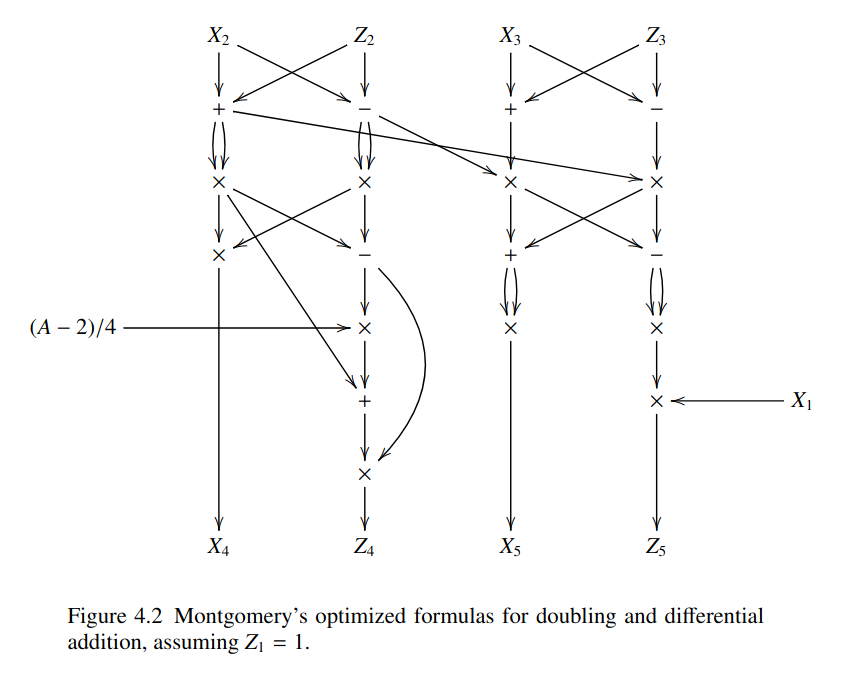
(See: ¹)

Ladder

One simple way to calculate $kP$ is as follows. Iterate over the bits of $k$ from most to least significant. If a bit $b=0$, set:

$$P\leftarrow 2P$$

If $b=1$, then set:

$$P\leftarrow 2P+P$$

Our addition formula works well when we have $P_n$ and $P_{n+1}$, and want to calculate $P_{2n+1}$, since the difference is $P_1=P$, a point we already know.

At each iteration, as we rise up to $P_k$, our final value, we want to keep this property, and keep the successive values around.

This, when $b=0$, we do:

$$(P_n,P_{n+1})\mapsto (P_{2n},P_{2n+1})$$

The first value comes from point doubling $P_n$, and the second from differential point addition, using the fact that the difference is $P_1$.

When $b=1$, we want to do:

$$(P_n,P_{n+1})\mapsto (P_{2n+1},P_{2n+2})$$

We can calculate the first value through point addition, and the second through point doubling.

In fact, if we define these two functions as ${\text{step}}_0$, and ${\text{step}}_1$ respectively, we notice that ${\text{step}}_1$ comes from swapping the input, and then the output. With:

$$\text{swap}(P,Q):=(Q,P)$$

We have:

$${\text{step}}_1=\text{swap};{\text{step}}_0;\text{swap}$$

Thus, an algorithm for doing our ladder would be:

for b in bits:
  if b == 1:
    swap(P, Q)
  (P, Q) = step0(P, Q)
  if b == 1:
    swap(P, Q)
return P

We can make this “constant-time”, by replacing our branching with a conditional swap:

for b in bits:
  cswap(b, P, Q)
  (P, Q) = step0(P, Q)
  cswap(b, P, Q)
return P

If we have two conditional swaps chained together

cswap(bits[i], P, Q)
cswap(bits[i - 1], P, Q)

Which happens between iterations, notice that this is effectively:

cswap(bits[i] ^ bits[i - 1], P, Q)

because of this, we can effectively do:

cswap(bits[N - 1], P, Q)
step0(P, Q)
cswap(bits[N - 1] ^ bits[N - 1], P, Q)
step0(P, Q)
...
cswap(bits[1] ^ bits[0], P, Q)
step0(P, Q)
cswap(bits[0], P, Q)

Noting that 0 ^ bits[N - 1] = bits[N - 1], we can effectively do:

swap := 0
for b in bits:
  swap ^= b
  cswap(swap, P, Q)
  swap = b
  step0(P, Q)
cswap(swap, P, Q)
return P

This allows us to efficiently compute whether or not we need to swap.

This is the gist of things, see the summary up top for more useable pseudo-code.

References

¹

Footnotes

1. [1] Bernstein, Daniel J., Lange, Tanja - Montgomery Curves and the Montgomery Ladder (2017) ↩ ↩² ↩³ ↩⁴